Image by Author

Linear Regression is the most popular and the first machine learning algorithm that a data scientist learns while starting their data science career. It is the most important supervised learning algorithm as it sets up the building blocks for all the other advanced Machine Learning algorithms. That is why we need to learn and understand this algorithm very clearly.

In this article, we will cover Linear Regression from scratch, its mathematical & geometric intuition, and its Python implementation. The only prerequisite is your willingness to learn and the basic knowledge of Python syntax. Let’s get started.

What is Linear Regression?

Linear Regression is a Supervised Machine Learning algorithm that is used to solve Regression problems. Regression models are used to predict a continuous output based on some other factors. E.g., Predicting the next month’s stock price of an organization by considering the profit margins, total market cap, yearly growth, etc. Linear Regression can also be used in applications like predicting the weather, stock prices, sales targets, etc.

As the name suggests, Linear Regression, it develops a linear relationship between two variables. The algorithm finds the best straight line (y=mx+c) that can predict the dependent variable(y) based on the independent variables(x). The predicted variable is called the dependent or target variable, and the variables used to predict are called the independent variables or features. If only one independent variable is used, then it is called Univariate Linear Regression. Otherwise, it is called Multivariate Linear Regression.

To simplify this article, we will only take one independent variable(x) so that we can easily visualize it on a 2D plane. In the next section, we will discuss its mathematical intuition.

Mathematical Intuition

Now we will understand Linear Regression’s geometry and its mathematics. Suppose we have a set of sample pairs of X and Y values,

We have to use these values to learn a function so that if we give it an unknown (x), it can predict a (y) based on the learnings. In regression, many functions can be used for prediction, but the linear function is the simplest among all.

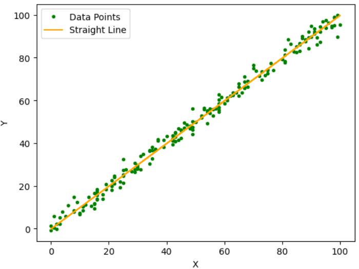
Fig.1 Sample Data Points | Image by Author

The main aim of this algorithm is to find the best-fit line among these data points, as indicated in the above figure, which gives the least residual error. The residual error is the difference between predicted and actual value.

Assumptions for Linear Regression

Before moving forward, we need to discuss some assumptions of Linear Regression that we need to be taken care of to get accurate predictions.

1. Linearity: Linearity means that the independent and dependent variables must follow a linear relationship. Otherwise, it will be challenging to obtain a straight line. Also, the data points must be independent of each other, i.e. the data of one observation does not depend on the data of another observation.
2. Homoscedasticity: It states that the variance of the residual errors must be constant. It means that the variance of the error terms should be constant and does not change even if the values of the independent variable change. Also, the errors in the model must follow a Normal Distribution.
3. No Multicollinearity: Multicollinearity means there is a correlation between the independent variables. So in Linear Regression, the independent variables must not be correlated with each other.

Hypothesis Function

We will hypothesise that a linear relationship will exist between our dependent variable(Y) and the independent variable(X). We can represent the linear relationship as follows.

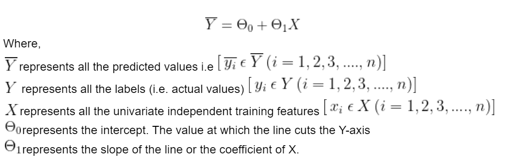
We can observe that the straight line depends on the parameters Θ0 and Θ1. So to get the best-fit line, we need to tune or adjust these parameters. These are also called the weights of the model. And to calculate these values, we will use the loss function, also known as the cost function. It calculates the Mean Squared Error between the predicted and actual values. Our goal is to minimize this cost function. The values of Θ0 and Θ1, in which the cost function is minimized, will form our best-fit line. The cost function is represented by (J) 

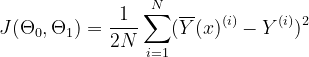
Where,

N is the total number of samples

The squared error function is chosen to handle the negative values (i.e. if the predicted value is less than the actual value). Also, the function is divided by 2 to ease the differentiation process.

Optimizer (Gradient Descent)

Optimizer is an algorithm that minimises the MSE by iteratively updating the model's attributes like weights or learning rate to achieve the best-fit line. In Linear Regression, the Gradient Descent algorithm is used to minimize the cost function by updating the values of Θ0 and Θ1. 

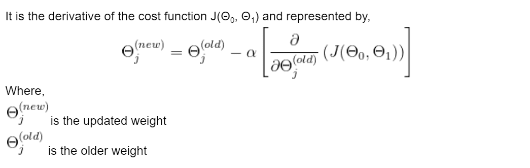
is a hyperparameter which is called the learning rate. It determines how much our weights are adjusted with respect to the gradient loss. The value of the learning rate should be optimal, not too high or too low. If it is too high, it is difficult for the model to converge at the global minimum, and if it is too small, it takes longer to converge. 

We will plot a graph between the Cost function and the Weights to find the optimum Θ0 and Θ1.

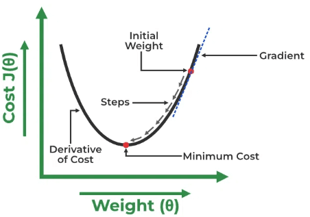
Fig.2 Gradient Descent Curve | Image by GeeksForGeeks

Initially, we will assign random values to Θ0 and Θ1, then calculate the cost function and gradient. For a negative gradient(a derivative of the cost function), we need to move in the direction of increasing Θ1 in order to reach the minima. And for a positive gradient, we must move backwards to reach the global minima. We aim to find a point at which the gradient almost equals zero. At this point, the value of the cost function is minimum.

By now, you have understood the working and mathematics of Linear Regression. The following section will see how to implement it from scratch using Python on a sample dataset.

Linear Regression Python Implementation

In this section, we will learn how to implement the Linear Regression algorithm from scratch only using fundamental libraries like Numpy, Pandas, and Matplotlib. We will implement Univariate Linear Regression, which contains only one dependent and one independent variable.

The dataset we will use contains about 700 pairs of (X, Y) in which X is the independent variable and Y is the dependent variable.  Ashish Jangra contributes this dataset, and you can download it from here.

Importing Libraries

# Importing Necessary Libraries
import pandas as pd
import numpy as np
import matplotlib.pyplot as plt
import matplotlib.axes as ax
from IPython.display import clear_output

Pandas reads the CSV file and gets the dataframe, while Numpy performs basic mathematics and statistics operations. Matplotlib is responsible for plotting graphs and curves.

Loading the Dataset

# Dataset Link:
# https://github.com/AshishJangra27/Machine-Learning-with-Python-GFG/tree/main/Linear%20Regression

df = pd.read_csv("lr_dataset.csv")
df.head()

# Drop null values
df = df.dropna()

# Train-Test Split
N = len(df)
x_train, y_train = np.array(df.X[0:500]).reshape(500, 1), np.array(df.Y[0:500]).reshape(
    500, 1
)
x_test, y_test = np.array(df.X[500:N]).reshape(N - 500, 1), np.array(
    df.Y[500:N]
).reshape(N - 500, 1)

First, we will get the dataframe df and then drop the null values. After that, we will split the data into training and testing x_train, y_train, x_test and y_test.

Building Model

class LinearRegression:
    def __init__(self):
        self.Q0 = np.random.uniform(0, 1) * -1  # Intercept
        self.Q1 = np.random.uniform(0, 1) * -1  # Coefficient of X
        self.losses = []  # Storing the loss of each iteration

    def forward_propogation(self, training_input):
        predicted_values = np.multiply(self.Q1, training_input) + self.Q0  # y = mx + c
        return predicted_values

    def cost(self, predictions, training_output):
        return np.mean((predictions - training_output) ** 2)  # Calculating the cost

    def finding_derivatives(self, cost, predictions, training_input, training_output):
        diff = predictions - training_output
        dQ0 = np.mean(diff)  # d(J(Q0, Q1))/d(Q0)
        dQ1 = np.mean(np.multiply(diff, training_input))  # d(J(Q0, Q1))/d(Q1)
        return dQ0, dQ1

    def train(self, x_train, y_train, lr, itrs):
        for i in range(itrs):
            # Finding the predicted values (Using the linear equation y=mx+c)
            predicted_values = self.forward_propogation(x_train)

            # Calculating the Loss
            loss = self.cost(predicted_values, y_train)
            self.losses.append(loss)

            # Back Propagation (Finding Derivatives of Weights)
            dQ0, dQ1 = self.finding_derivatives(
                loss, predicted_values, x_train, y_train
            )

            # Updating the Weights
            self.Q0 = self.Q0 - lr * (dQ0)
            self.Q1 = self.Q1 - lr * (dQ1)

            # It will dynamically update the plot of the straight line
            line = self.Q0 + x_train * self.Q1
            clear_output(wait=True)
            plt.plot(x_train, y_train, "+", label="Actual values")
            plt.plot(x_train, line, label="Linear Equation")
            plt.xlabel("Train-X")
            plt.ylabel("Train-Y")
            plt.legend()
            plt.show()
        return (
            self.Q0,
            self.Q1,
            self.losses,
        )  # Returning the final model weights and the losses

We have created a class named LinearRegression() in which all the required functions are built. 

__init__ : It is a constructor and will initialize the weights with random values when the object of this class is created.

forward_propogation(): This function will find the predicted output using the equation of the straight line.

cost(): This will calculate the residual error associated with the predicted values.

finding_derivatives(): This function calculates the derivative of the weights, which can later be used to update the weights for minimum errors.

train(): This function will take input from the training data, learning rate and the total number of iterations. It will update the weights using back-propagation until the specified number of iterations. At last, it will return the weights of the best-fit line.

Training the Model

lr = 0.0001  # Learning Rate
itrs = 30  # No. of iterations
model = LinearRegression()
Q0, Q1, losses = model.train(x_train, y_train, lr, itrs)

# Output No. of Iteration vs Loss
for itr in range(len(losses)):
    print(f"Iteration = {itr+1}, Loss = {losses[itr]}")

Output:

Iteration = 1, Loss = 6547.547538061649
Iteration = 2, Loss = 3016.791083711492
Iteration = 3, Loss = 1392.3048668536044
Iteration = 4, Loss = 644.8855797373262
Iteration = 5, Loss = 301.0011032250385
Iteration = 6, Loss = 142.78129818453215
.
.
.
.
Iteration = 27, Loss = 7.949420840198964
Iteration = 28, Loss = 7.949411555664398
Iteration = 29, Loss = 7.949405538972356
Iteration = 30, Loss = 7.949401025888949

You can observe that in the 1st iteration, the loss is maximum, and in the subsequent iterations, this loss decreases and reaches its minimum value at the end of the 30th iteration.

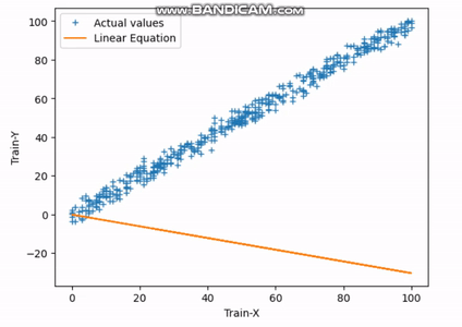
Fig.3 Finding Best-fit Line | Image by Author

The above gif indicates how the straight line reaches its best-fit line after completing the 30th iteration.

Final Prediction

# Prediction on test data
y_pred = Q0 + x_test * Q1
print(f"Best-fit Line: (Y = {Q1}*X + {Q0})")

# Plot the regression line with actual data pointa
plt.plot(x_test, y_test, "+", label="Data Points")
plt.plot(x_test, y_pred, label="Predited Values")
plt.xlabel("X-Test")
plt.ylabel("Y-Test")
plt.legend()
plt.show()

This is the final equation of the best-fit line.

Best-fit Line: (Y = 1.0068007107347927*X + -0.653638673779529)

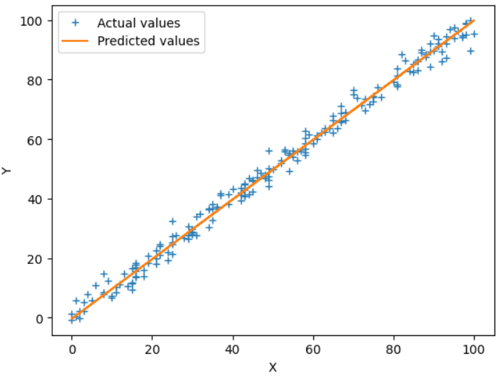
Fig.4 Actual vs Predicted Output | Image by Author

The above plot shows the best-fit line (orange) and actual values (blue +) of the test set. You can also tune the hyperparameters, like the learning rate or the number of iterations, to increase the accuracy and precision.

Linear Regression (Using Sklearn Library)

In the previous section, we have seen how to implement Univariate Linear Regression from scratch. But there is also a built-in library by sklearn that can be directly used to implement Linear Regression. Let’s briefly discuss how we can do it.

We will use the same dataset, but if you want, you can use a different one also. You need to import two extra libraries as follows.

# Importing Extra Libraries
from sklearn.linear_model import LinearRegression
from sklearn.model_selection import train_test_split

Loading Dataset

df = pd.read_csv("lr_dataset.csv")

# Drop null values
df = df.dropna()

# Train-Test Split
Y = df.Y
X = df.drop("Y", axis=1)
x_train, x_test, y_train, y_test = train_test_split(
    X, Y, test_size=0.25, random_state=42
)

Earlier, we had to perform the train-test split using the numpy library manually. But now we can use sklearn's train_test_split() to directly divide the data into the training and testing sets just by specifying the testing size.

Model Training and Predictions

model = LinearRegression()
model.fit(x_train, y_train)
y_pred = model.predict(x_test)

# Plot the regression line with actual data points
plt.plot(x_test, y_test, "+", label="Actual values")
plt.plot(x_test, y_pred, label="Predicted values")
plt.xlabel("X")
plt.ylabel("Y")
plt.legend()
plt.show()

Now, we don’t have to write the codes for forward propagation, backward propagation, cost function, etc. We can now directly use the LinearRegression() class and train the model on the input data. Below is the plot obtained on the test data from the trained model. The results are similar to when we implemented the algorithm on our own.

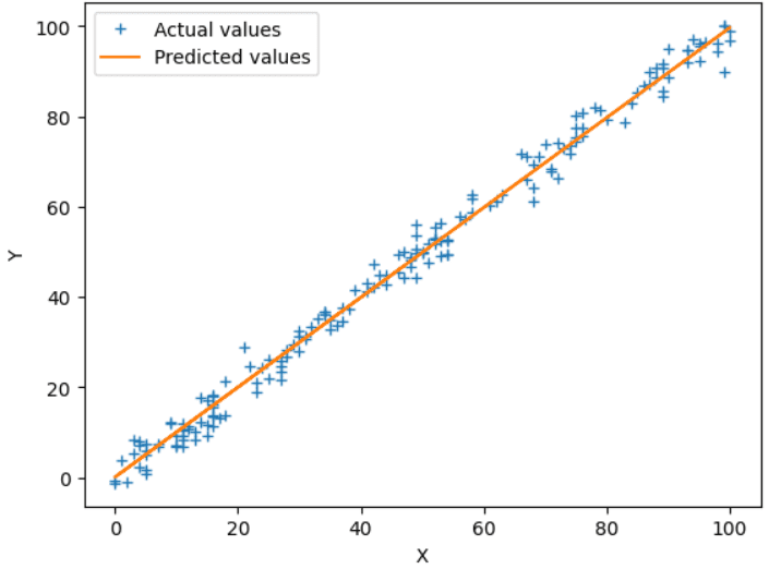
Fig.5 Sklearn Model Output | Image by Author

References

1. GeeksForGeeks:  ML Linear Regression

Wrapping it Up

Google Colab Link for the Complete Code - Linear Regression Tutorial Code

In this article, we have thoroughly discussed what Linear Regression is, its mathematical intuition and its Python implementation both from scratch and from using sklearn’s library. This algorithm is straightforward and intuitive, so it helps beginners to lay a solid foundation as well as helps to gain practical coding skills to make accurate predictions using Python.

Thanks for reading.
 
 
Aryan Garg is a B.Tech. Electrical Engineering student, currently in the final year of his undergrad. His interest lies in the field of Web Development and Machine Learning. He have pursued this interest and am eager to work more in these directions.