Missing Value Imputation – A Review

By Kathrin Melcher, Data Scientist at KNIME, and Rosaria Silipo, Principal Data Scientist at KNIME

Missing values occur in all kinds of datasets from industry to academia. They can be represented differently  - sometimes by a question mark, or  -999, sometimes by “n/a”, or by  some other dedicated number or character. Detecting and handling missing values in the correct way is important, as they can impact the results of the analysis, and there are algorithms that can’t handle them. So what is the correct way?

 

How to choose the correct strategy

 
Two common approaches to imputing missing values is to replace all missing values with either a fixed value, for example zero, or with the mean of all available values. Which approach is better?

Let’s see the effects on two different case studies:

• Case Study 1: threshold-based anomaly detection on sensor data
• Case Study 2: a report of customer aggregated data

Case Study 1: Imputation for threshold-based anomaly detection

In a classic threshold-based solution for anomaly detection, a threshold, calculated from the mean and variance of the original data, is applied to the sensor data to generate an alarm. If the missing values are imputed with a fixed value, e.g. zero, this will affect the calculation of the mean and variance used for the threshold definition. This would likely lead to a wrong estimate of the alarm threshold and to some expensive downtime.

Here imputing the missing values with the mean of the available values is the right way to go.

Case Study 2: Imputation for aggregated customer data

In a classic reporting exercise on customer data, the number of customers and the total revenue for each geographical area of the business needs to be aggregated and visualized, for example via bar charts. The customer dataset has missing values for those areas where the business has not started or has not picked up and no customers and no business have been recorded yet. In this case, using the mean value of the available numbers to impute the missing values would make up customers and revenues where neither customers nor revenues are present.

The right way to go here is to impute the missing values with a fixed value of zero. 

In both cases, it is our knowledge of the process that suggests to us the right way to proceed in imputing missing values. In the case of sensor data, missing values are due to a malfunctioning of the measuring machine and therefore real numerical values are just not recorded. In the case of the customer dataset, missing values appear where there is nothing to measure yet.

You see already from these two examples, that there is no panacea for all missing value imputation problems and clearly we can’t provide an answer to the classic question: “which strategy is correct for missing value imputation for my dataset?” The answer is too dependent on the domain and the business knowledge.

We can however provide a review of the most commonly used techniques to:

• Detect whether the dataset contains missing values and of which type, 
• Impute the missing values. 

 

Detecting Missing Values and their Type

 
Before trying to understand where the missing values come from and why, we need to detect them. Common encodings for missing values are n/a, NA,  -99, -999, ?, the empty string, or any other placeholder. When you open a new dataset, without instructions, you need to recognize if any such placeholders have been used to represent missing values.

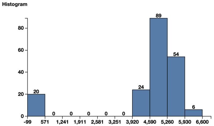
Histograms are a great tool to find the placeholder character, if any. 

• For numerical values many datasets use a value far away from the distribution of the data to represent the missing values. A classic is the -999 for data in the positive range. In figure 1, the histogram shows most of the data in the range [3900-6600] are nicely Gaussian-distributed. The little bar towards the left around -99 looks quite displaced with respect to the rest of the data and could be a candidate for a placeholder number used to indicate missing values.
• Usually, for nominal data, it is easier to recognize the placeholder for missing values, since the string format allows us to write some reference to a missing value, like “unknown” or “N/A”. The histogram can also help us here. For nominal data, bins with non fitting values could be an indicator of the missing value placeholder. 

 

This step, to detect placeholder characters/numbers representing missing values, belongs to the data exploration phase, before the analysis starts. After detecting this placeholder character for missing values and prior to the real analysis, the missing value must be formatted properly, according to the data tool in use. 

An interesting academic exercise consists in qualifying the type of the missing values. Missing values are usually classified into three different types [1][2].
 

• Missing Completely at Random (MCAR)
  Definition: The probability of an instance being missing does not depend on known values or the missing value itself. 
  Example: A data table was printed with no missing values and someone accidentally dropped some ink on it so that some cells are no longer readable [2]. Here, we could assume that the missing values follow the same distribution as the known values.

• Missing at Random (MAR)
  Definition: The probability of an instance being missing may depend on known values but not on the missing value itself.
  Sensor Example: In the case of a temperature sensor, the fact that a value is missing doesn’t depend on the temperature, but might be dependent on some other factor, for example on the battery charge of the thermometer. 
  Survey example: Whether or not someone answers a question - e.g. about age- in a survey doesn’t depend on the answer itself, but may depend on the answer to another question, i.e. gender female.  

• Not Missing at Random (NMAR)
  Definition: the probability of an instance being missing could depend on the value of the variable itself.
  Sensor example: In the case of a temperature sensor, the sensor doesn’t work properly when it is colder than 5°C. 
  Survey example: Whether or not someone answers a question - e.g. number of sick days - in a survey does depend on the answer itself - as it could be for some overweight people. 

Only the knowledge of the data collection process and the business experience can tell whether the missing values we have found are of type MAR, MCAR, or NMAR. 

For this article, we will focus only on MAR or MCAR types of missing values. Imputing NMAR missing values is more complicated, since additional factors to just statistical distributions and statistical parameters have to be taken into account.

 

Different Methods to Handle Missing Values

 
The many methods, proposed over the years, to handle missing values can be separated in two main groups: deletion and imputation. 

 

Deletion Methods

 
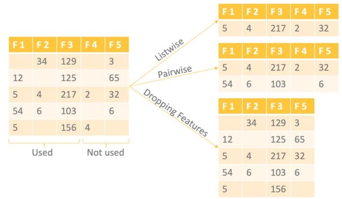
There are three common deletion approaches: listwise deletion, pairwise deletion, and dropping features. 

• Listwise Deletion: Delete all rows where one or more values are missing. 
• Pairwise Deletion: Delete only the rows that have missing values in the columns used for the analysis. It is only recommended to use this method if the missing data are MCAR.
• Dropping Features: Drop entire columns with more missing values than a given threshold, e.g. 60%.

 

Imputation Methods

 
The idea behind the imputation approach is to replace missing values with other sensible values. As you always lose information with the deletion approach when dropping either samples (rows) or entire features (columns), imputation is often the preferred approach. 

The many imputation techniques can be divided into two subgroups: single imputation or multiple imputation. 

In single imputation, a single / one imputation value for each of the missing observations is generated.  The imputed value is treated as the true value, ignoring the fact that no imputation method can provide the exact value. Therefore, single imputation does not reflect the uncertainty of the missing values.

In multiple imputation, many imputed values for each of the missing observations are generated. This means many complete datasets with different imputed values are created. The analysis (e.g. training a linear regression to predict a target column) is performed on each of these datasets and the results are polled. Creating multiple imputations, as opposed to single imputations, accounts for the statistical uncertainty in the imputations [3][4]. 

 

Single Imputation

 
Most imputation methods are single imputation methods, following three main strategies: replacement by existing values, replacement by statistical values, and replacement by predicted values. Depending on the values used for each one of these strategies, we end up with methods that work on numerical values only and methods that work on both numerical and nominal columns. These methods are summarized in Table 1 and explained below.

Replacement by:	Numerical Features Only	Numerical and Nominal Features
Existing values	Minimum / Maximum	Previous / Next / Fixed
Statistical values	(Rounded) Mean / Median / Moving Average, Linear / Average Interpolation	Most Frequent
Predicted values	Regression Algorithms	Regression & Classification Algorithms, k-Nearest Neighbours

Table 1: Single imputation methods for numerical features only and for numerical and nominal features, based on existing values, statistical measures, and predicted values.
 

Fixed Value 

Fixed value imputation is a general method that works for all data types and consists of substituting the missing value with a fixed value. The aggregated customer example we mentioned at the beginning of this article uses fixed value imputation for numerical values. As an example of using fixed value imputation on nominal features, you can impute the missing values in a survey with “not answered”.

Minimum / Maximum Value

If you know that the data has to fit a given range [minimum, maximum], and if you know from the data collection process that  the measuring system stops recording and the signal saturates beyond one of such boundaries, you can use the range minimum or maximum as the replacement value for missing values. For example, if in the monetary exchange a minimum price has been reached and the exchange process has been stopped, the missing monetary exchange price can be replaced with the minimum value of the law’s exchange boundary.

(Rounded) Mean / Median Value / Moving Average

Other common imputation methods for numerical features are mean, rounded mean, or median imputation. In this case, the method substitutes the missing value with the mean, the rounded mean, or the median value calculated for that feature on the whole dataset. In the case of a high number of outliers in your dataset, it is recommended to use the median instead of the mean. 

Most Frequent Value

Another common method that works for both numerical and nominal features uses the most frequent value in the column to replace the missing values.

Previous / Next Value 

There are special imputation methods for time series or ordered data. These methods take into account the sorted nature of the dataset, where close values are probably more similar than distant values. A common approach for imputing missing values in time series substitutes the next or previous value to the missing value in the time series. This approach works for both numerical and nominal values.

Linear / Average Interpolation

Similarly to the previous/next value imputation, but only applicable to numerical values, is linear or average interpolation, which is calculated between the previous and next available value, and substitutes the missing value. Of course, as for all operations on ordered data, it is important to sort the data correctly in advance, e.g. according to a timestamp in the case of time series data.

K Nearest Neighbors 

The idea here is to look for the k closest samples in the dataset where the value in the corresponding feature is not missing and to take the feature value occurring most frequently in the group as a replacement for the missing value.

Missing Value Prediction

Another common option for single imputation is to train a machine learning model to predict the imputation values for feature x based on the other features. The rows without missing values in feature x are used as a training set and the model is trained based on the values in the other columns. Here we can use any classification or regression model, depending on the data type of the feature. After training, the model is applied to all samples with the feature missing value to predict its most likely value.

In the case of missing values in more than one feature column, all missing values are first temporarily imputed with a basic imputation method, e.g. the mean value. Then the values for one column are set back to missing. The model is then trained and applied to fill in the missing values. In this way, one model is trained for each feature with missing values, until all missing values are imputed by a model.

 

Multiple Imputation

 
Multiple imputation is an imputation approach stemming from statistics. Single imputation methods have the disadvantage that they don’t consider the uncertainty of the imputed values. This means they recognize the imputed values as actual values not taking into account the standard error, which causes bias in the results [3][4].

An approach that solves this problem is multiple imputation where not one, but many imputations are created for each missing value. This means filling in the missing values multiple times, creating multiple “complete” datasets [3][4].

A number of algorithms have been developed for multiple imputation. One well known algorithm is Multiple Imputation by Chained Equation (MICE).

Multiple Imputation by Chained Equations (MICE)

Multiple Imputation by Chained Equations (MICE) is a robust, informative method for dealing with missing values in datasets. MICE operates under the assumption that the missing data are Missing At Random (MAR) or Missing Completely At Random (MCAR) [3].

The procedure is an extension of the single imputation procedure by “Missing Value Prediction” (seen above): this is step 1. However, there are two additional steps in the MICE procedure.

Step 1: This is the process as in the imputation procedure by “Missing Value Prediction” on a subset of the original data. One model is trained to predict the missing values in one feature, using the other features in the data row as the independent variables for the model. This step is repeated for all features. This is a cycle or iteration. 

Step 2: Step 1 is repeated k times, each time using the most recent imputations for the independent variables, until convergence is reached. Most often, k=10 cycles are sufficient.

Step 3: The whole process is repeated N times on N different random subsets. The resulting N models will be slightly different, and will produce N slightly different predictions for each missing value.

The analysis, e.g. training a linear regression for a target variable, is now performed on each one of the N final datasets. Finally the results are combined, often this is also called pooling.

This provides more robust results than by single imputation alone. Of course, the downside of such robustness is the increase in computational complexity.

 

Comparing Imputation Techniques

 
Many imputation techniques. Which one to choose? 

Sometimes we should already know what the best imputation procedure is, based on our knowledge of the business and of the data collection process. Sometimes, though, we have no clue so we just try a few different options and see which one works best.

To define “best”, we need a task. The procedure that gets the best performance as regards to our specified task is the one that works “best”. And this is exactly what we have tried to do in this article: define a task, define a measure of success for the task, experiment with a few different missing value imputation procedures, and compare the results to find the most suitable one. 

Let’s limit our investigation to classification tasks. The measures for success will be the accuracy and the Cohen’s Kappa of the model predictions. The accuracy is a clear measure of task success in case of datasets with balanced classes. However, Cohen’s Kappa, though less easy to read and to interpret, represents a better measure of success for datasets with unbalanced classes.

We implemented two classification tasks, each one on a dedicated dataset:

• Churn prediction on the Churn prediction dataset (3333 rows, 21 columns)
• Income prediction on the Census income dataset (32561 rows, 15 columns)

For both classification tasks we chose a simple decision tree, trained on 80% of the original data and tested on the remaining 20%. The point here is to compare the effects of different imputation methods, by observing possible improvements in the model performance when using one imputation method rather than another.

We repeated each classification task four times: on the original dataset, and after introducing 10%, 20%, and 25% missing values of type MCAR across all input features. This means we randomly removed values across the dataset and transformed them into missing values.

Each time, we experimented with four different missing value imputation techniques (Fig. 3).

• Deletion: Listwise deletion (blue)
• 0 imputation: Fixed value imputation with zero (orange)
• Mean - most frequent: Mean imputation for numerical values and most frequent value imputation for nominal values (green)
• Linear regr - kNN: Missing value prediction with linear regression for numerical values and kNN for nominal values (red)

Figure 3 compares the accuracies and Cohen’s Kappas of the decision trees after the application of the four selected imputation methods on the original dataset and on the versions with artificially inserted missing values. 

 

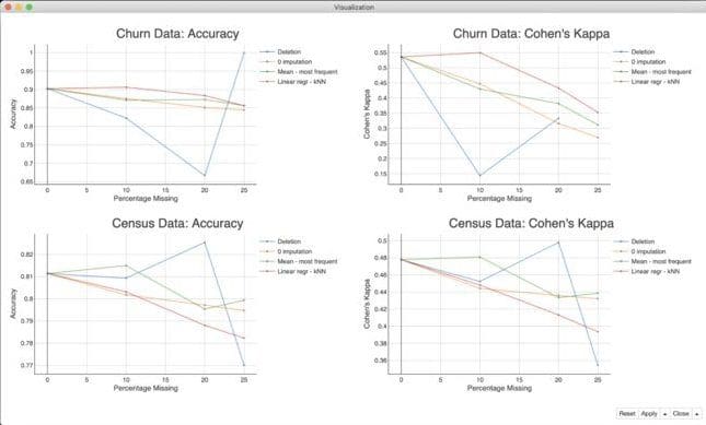
For three of the four imputation methods, we can see the general trend that the higher the percentage of missing values the lower the accuracy and the Cohen’s Kappa, of course. The exception is the deletion approach (blue lines). 

In addition we can not see a clear winner approach. This sustains our statement that the best imputation method depends on the use case and on the data.

The churn dataset is a dataset with unbalanced class churn, where class 0 (not churning) is much more numerous than class 1 (churning). The listwise deletion leads here to really small datasets and makes it impossible to train a meaningful model. In this example we end up with only one row in the test set, which is by chance predicted correctly (blue line). This explains the 100% accuracy and the missing Cohen’s Kappa.

All other imputation techniques obtain more or less the same performance for the decision tree on all variants of the dataset, in terms of both accuracy and Cohen’s Kappa. The best results, though, are obtained by the missing value prediction approach, using linear regression and kNN. 

The Census income dataset is a larger dataset compared to the churn prediction dataset, where the two income classes, <=50K and  >50K, are also unbalanced. The plots in Figure 3 show that the mean and most frequent imputation outperforms the missing value prediction approach as well as the 0 imputation, in terms of accuracy and Cohen’s Kappa. In case of the deletion approach the results for the Census dataset are unstable and dependent on the subsets resulting from the listwise deletion. In the setup used here, deletion (blue line) improves the performance for small percentages of missing values, but leads to a poor performance for 25% or more missing values. 

 

The Comparison Application

 
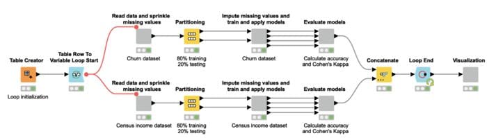
The application to compare all described techniques and generate the charts in figure 3 was developed using KNIME Analytics Platform (Fig. 4).

Here a loop iterates over the four variants of the datasets: with 0%, 10%, 20% and 25% missing values. At each iteration, each one of the two branches within the loop implements one of the two classification tasks: churn prediction or income prediction. In particular each branch:

• Reads the dataset and sprinkles missing data over it in the percentage set for this loop iteration
• Randomly partitions the data in a 80%-20% proportion to respectively train and test the decision tree for the selected task
• Imputes the missing values according to the four selected methods and trains and tests the decision tree
• Calculates the accuracies and Cohen’s Kappas for the different models. 

Afterwards the two loop branches are concatenated and the Loop End node  collects the performance results from the different iterations, before they get visualized through the “Visualize results” component 

• You can download the workflow, Comparing Missing Value Handling Methods, from the KNIME Hub.

  

The component named “Impute missing values and train and apply models” is the one of interest here. Its content is shown in figure 5: Four branches, as it was to be expected, one for each imputation technique. 

The top three branches implement the listwise deletion (“deletion”), fixed value imputation with zero (“0 imputation”), statistical measure imputation using the mean for numerical features and the most frequent value for nominal features (“Mean - most frequent”).

The last branch implements the missing value prediction imputation, using a linear regression for numerical features and a kNN for nominal features (“linear regre - kNN”).

 

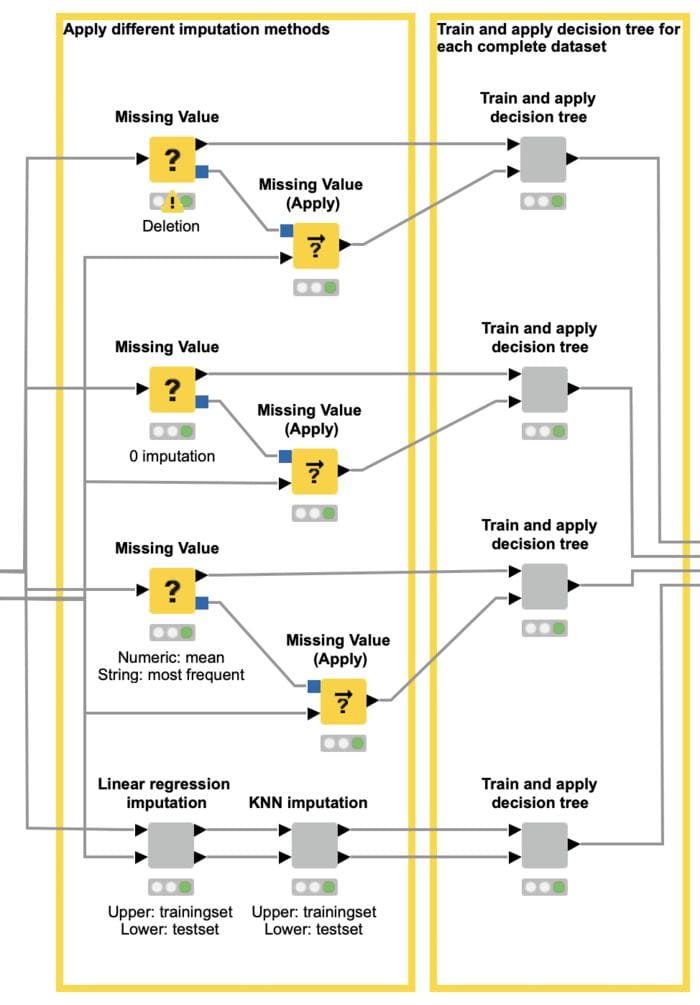
Let’s conclude with a few words to describe the Missing Value node, simple yet effective. The Missing Value node offers most of the introduced single imputation techniques (Only the kNN and predictive model approach are not available). Here you can impute missing values according to a selected strategy across all datasets or column (feature) by column (feature).  

 

Multiple Imputation in KNIME Analytics Platform

 
In the workflow, Comparing Missing Value Handling Methods, shown above, we saw how different single imputation methods can be applied in KNIME Analytics Platform. And it would be clearly possible to build a loop to implement a multiple imputation approach using the MICE algorithm. One advantage of KNIME Analytics Platform though is that we don’t have to reinvent the wheel, but we can integrate algorithms available in Python and R easily.

The “mice” package in R allows you to impute mixes of continuous, binary, unordered categorical and ordered categorical data and selecting from many different algorithms, creating many complete datasets. [5]

In Python the “IterativeImputar” function was inspired by the MICE algorithm. It performs the same round-robin fashion of iterating many times through the different columns, but creates only one imputed dataset. By using different random seeds, multiple complete datasets can be created. [6]

In general it is still an open problem how useful single vs. multiple imputation is in the context of prediction and classification, when the user is not interested in measuring uncertainty due to missing values.

The workflow, Multiple Imputation for Missing Values, in Figure 7 shows an example for multiple imputation using the R “mice” package to create five complete datasets. 

  

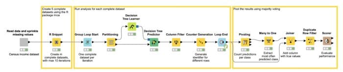
The workflow reads the census dataset after 25% of the values of the input features were replaced with missing values. In the R snippet node, the R “mice” package is loaded and applied to create the five complete datasets. In addition, an index is added to each row identifying the different complete datasets.

• You can download the workflow, Multiple Imputation for Missing Values, from the KNIME Hub.

In the next step, a loop processes the different complete datasets, by training and applying a decision tree in each iteration. In the last part of the workflow, the predicted results are polled by counting how often each class has been predicted and extracting the majority predicted class. Finally the result is evaluated using the Scorer node. On the Iris “mice” imputed dataset, the model reached an accuracy of 83.867%. In comparison, the single imputation methods reached between 77% and 80% accuracy on the dataset with 25% missing values. 

 

Wrapping up

 
All datasets have missing values. It is necessary to know how to deal with them. Should we remove the data rows entirely or substitute some reasonable value as the missing value?

In this blog post, we described some common techniques that can be used to delete and impute missing values. We then implemented four most representative techniques, and compared the effect of four of them in terms of performances on two different classification problems with a progressive number of missing values.

Summarizing, we can reach the following conclusions.

Use listwise deletion (“deletion”) carefully, especially on small datasets. When removing data, you are removing information. Not all datasets have redundant information to spare! We have seen this dramatic effect in the churn prediction task.

When using fixed value imputation, you need to know what that fixed value means in the data domain and in the business problem. Here, you are injecting arbitrary information into the data, which can bias the predictions of the final model. 

If you want to impute missing values without prior knowledge it is hard to say which imputation method works best, as it is heavily dependent on the data itself.

A small last disclaimer here to conclude. All results obtained here refer to these two simple tasks, to a relatively simple decision tree, and to small datasets. The same results might not hold for more complex situations. 

In the end, nothing beats prior knowledge of the task and of the data collection process!

 
References:

[1] Peter Schmitt, Jonas Mandel and Mickael Guedj , “A comparison of six methods for missing data imputation”, Biometrics & Biostatistics
[2] ] M.R. Berthold, C. Borgelt, F. Höppner, F. Klawonn, R. Silipo, “Guide to Intelligent Data Science”, Springer, 2020
[3] lissa J. Azur, Elizabeth A. Stuart, Constantine Frangakis, and Philip J. Leaf 1, “Multiple imputation by chained equations: what is it and how does it work?” Link: https://www.ncbi.nlm.nih.gov/pmc/articles/PMC3074241/
[4] Shahidul Islam Khan, Abu Sayed Md Latiful Hoque,” SICE: an improved missing data imputation technique”, Link: https://link.springer.com/content/pdf/10.1186/s40537-020-00313-w.pdf
[5] Python documentation. Link: https://scikit-learn.org/stable/modules/impute.html
[6] Census Income Dataset: https://archive.ics.uci.edu/ml/datasets/Census+Income

 
Related:

• Easy Guide To Data Preprocessing In Python
• Automated Machine Learning: Just How Much?
• How to Deal with Missing Values in Your Dataset