Most Popular Distance Metrics Used in KNN and When to Use Them

By Sarang Anil Gokte, Praxis Business School

 

Introduction

 
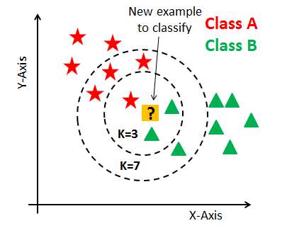
KNN is the most commonly used and one of the simplest algorithms for finding patterns in classification and regression problems. It is an unsupervised algorithm and also known as lazy learning algorithm. It works by calculating the distance of 1 test observation from all the observation of the training dataset and then finding K nearest neighbors of it. This happens for each and every test observation and that is how it finds similarities in the data. For calculating distances KNN uses a distance metric from the list of available metrics.

 

 

Distance Metrics

 
For the algorithm to work best on a particular dataset we need to choose the most appropriate distance metric accordingly. There are a lot of different distance metrics available, but we are only going to talk about a few widely used ones. Euclidean distance function is the most popular one among all of them as it is set default in the SKlearn KNN classifier library in python.

So here are some of the distances used:

 
Minkowski Distance – It is a metric intended for real-valued vector spaces. We can calculate Minkowski distance only in a normed vector space, which means in a space where distances can be represented as a vector that has a length and the lengths cannot be negative.

There are a few conditions that the distance metric must satisfy:

1. Non-negativity: d(x, y) >= 0
2. Identity: d(x, y) = 0 if and only if x == y
3. Symmetry: d(x, y) = d(y, x)
4. Triangle Inequality: d(x, y) + d(y, z) >= d(x, z)

 

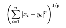
This above formula for Minkowski distance is in generalized form and we can manipulate it to get different distance metrices.

The p value in the formula can be manipulated to give us different distances like:

• p = 1, when p is set to 1 we get Manhattan distance
• p = 2, when p is set to 2 we get Euclidean distance

 
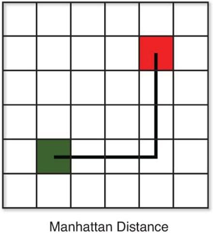
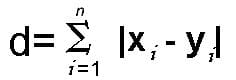
Manhattan Distance – This distance is also known as taxicab distance or city block distance, that is because the way this distance is calculated. The distance between two points is the sum of the absolute differences of their Cartesian coordinates.

 

As we know we get the formula for Manhattan distance by substituting p=1 in the Minkowski distance formula.

 

Suppose we have two points as shown in the image the red(4,4) and the green(1,1).

And now we have to calculate the distance using Manhattan distance metric.

We will get,

d = |4-1| + |4-1| = 6

This distance is preferred over Euclidean distance when we have a case of high dimensionality.

 
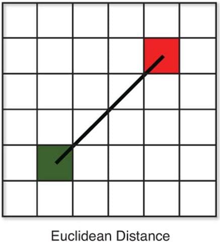
Euclidean Distance – This distance is the most widely used one as it is the default metric that SKlearn library of Python uses for K-Nearest Neighbour. It is a measure of the true straight line distance between two points in Euclidean space.

 

It can be used by setting the value of p equal to 2 in Minkowski distance metric.

 

Now suppose we have two point the red (4,4) and the green (1,1).

And now we have to calculate the distance using Euclidean distance metric.

We will get,

4.24

 
Cosine Distance – This distance metric is used mainly to calculate similarity between two vectors. It is measured by the cosine of the angle between two vectors and determines whether two vectors are pointing in the same direction. It is often used to measure document similarity in text analysis. When used with KNN this distance gives us a new perspective to a business problem and lets us find some hidden information in the data which we didn’t see using the above two distance matrices.

It is also used in text analytics to find similarities between two documents by the number of times a particular set of words appear in it.

Formula for cosine distance is:

 

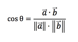
Using this formula we will get a value which tells us about the similarity between the two vectors and 1-cosΘ will give us their cosine distance.

Using this distance we get values between 0 and 1, where 0 means the vectors are 100% similar to each other and 1 means they are not similar at all.

 
Jaccard Distance - The Jaccard coefficient is a similar method of comparison to the Cosine Similarity due to how both methods compare one type of attribute distributed among all data.  The Jaccard approach looks at the two data sets and finds the incident where both values are equal to 1.  So the resulting value reflects how many 1 to 1 matches occur in comparison to the total number of data points. This is also known as the frequency that 1 to 1 match, which is what the Cosine Similarity looks for, how frequent a certain attribute occurs.

It is extremely sensitive to small samples sizes and may give erroneous results, especially with very small data sets with missing observations.

The formula for Jaccard index is:

 

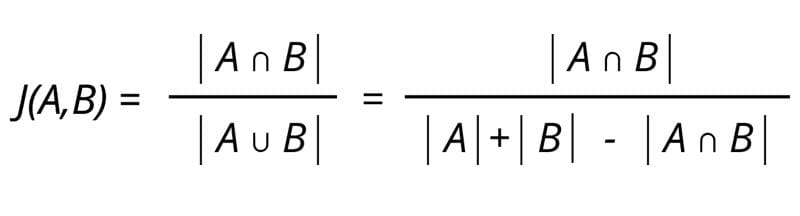
Jaccard distance is the complement of the Jaccard index and can be found by subtracting the Jaccard Index from 100%, thus the formula for Jaccard distance is:

D(A,B) = 1 – J(A,B)

 
Hamming Distance - Hamming distance is a metric for comparing two binary data strings. While comparing two binary strings of equal length, Hamming distance is the number of bit positions in which the two bits are different. The Hamming distance method looks at the whole data and finds when data points are similar and dissimilar one to one.  The Hamming distance gives the result of how many attributes were different.

This is used mostly when you one-hot encode your data and need to find distances between the two binary vectors.

Suppose we have two strings “ABCDE” and “AGDDF” of same length and we want to find the hamming distance between these. We will go letter by letter in each string and see if they are similar or not like first letters of both strings are similar, then second is not similar and so on.

ABCDE and AGDDF

When we are done doing this we will see that only two letters marked in red were similar and three were dissimilar in the strings. Hence, the Hamming Distance here will be 3. Note that larger the Hamming Distance between two strings, more dissimilar will be those strings (and vice versa).

 
References:

1. Sklearn distance metrics documentation
2. KNN in python
3. 4 Distance Measures for Machine Learning
4. Importance of Distance Metrics in Machine Learning Modelling
5. Different Types of Distance Metrics used in Machine Learning
6. Jaccard Index / Similarity Coefficient
7. Exercise for calculating Hamming and Jaccard Distances
8. Wikipedia
9. Cosine Similarity
10. Effects of Distance Measure Choice on KNN Classifier Performance - A Review

 
 
Bio: Sarang Anil Gokte is a Postgraduate Student at Praxis Business School.

Related:

• Introduction to the K-nearest Neighbour Algorithm Using Examples
• How to Explain Key Machine Learning Algorithms at an Interview
• /2020/10/exploring-brute-force-nearest-neighbors-algorithm.html