5 Things That Make My Job as a Data Scientist Easier

By Shree Vandana, Data Scientist

Photo by Boitumelo Phetla on Unsplash

1. Time Series Data Processing with Pandas

 
 
If you work with time series data, chances are you have spent a significant amount of time accounting for missing records or aggregating data at a particular temporal granularity either via SQL queries or writing custom functions. Pandas has a very efficient resample function that can help you process the data at a particular frequency by simply setting the DataFrame index to be the timestamp column.

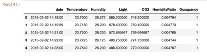
I am going to use the room occupancy dataset to give an example of this function. You can find the dataset here. This dataset records observations at a minute level.

import pandas as pd
data = pd.read_csv('occupancy_data/datatest.txt').reset_index(drop = True)
data.head(5)

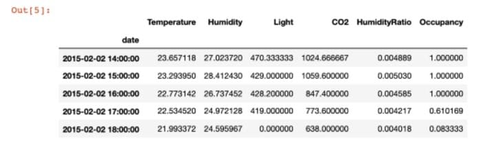
First, I show a simple aggregation one can do to get metrics at an hourly level.

data.index = pd.to_datetime(data['date'])
pd.DataFrame(data.resample('H').agg({'Temperature':'mean',
                                     'Humidity':'mean',
                                     'Light':'last',
                                     'CO2':'last',
                                     'HumidityRatio' : 'mean',
                                     'Occupancy' : 'mean'})).head(5)

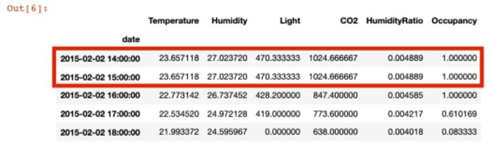
Though this dataset is not sparse, in the real world one often encounters data which has missing records. It is important to account for those records since you might want to put in 0 values if there were no records or use the previous or next time steps for imputation. Below, I removed records for hour 15 to show how you can use the hour 14 timestamp to impute the missing value:

data = pd.read_csv('occupancy_data/datatest.txt').reset_index(drop = True)data_missing_records = data[~(pd.to_datetime(data.date).dt.hour == 15)].reset_index(drop = True)data_missing_records.index = pd.to_datetime(data_missing_records['date'])data_missing_records.resample('H', base = 1).agg({'Temperature':'mean',
        'Humidity':'mean',
        'Light':'last',
        'CO2':'last',
        'HumidityRatio' : 'mean',
         'Occupancy' : 'mean'}).fillna(method  = 'ffill').head(5)

2. Fast Visualization via Plotly Express

 
 
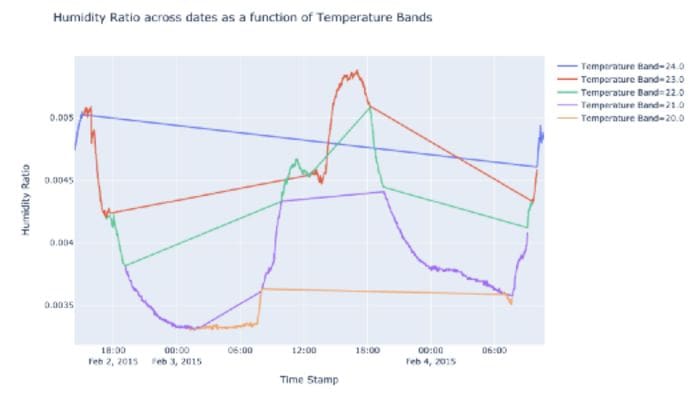
From analysis to model training to model reporting, visualizations are often required. Especially with time series graphs, I noticed I was spending a lot of time trying to customize the size and angle of my x-axis ticks in matplotlib. After I switched to using Plotly Express, I cut down the time I spent in making graphs looking cleaner/crisper by around 70%. And if I want to implement specific details in my visuals I can still do that by using Plotly Graph Objects. Additionally, Plotly offers a lot of easy options via Express like setting group colors in plots which results in more powerful visualizations.

import plotly.express as px
data['Temp_Bands'] = np.round(data['Temperature'])
fig = px.line(data, x = 'date',
              y = 'HumidityRatio',
              color = 'Temp_Bands',
             title = 'Humidity Ratio across dates as a function of
             Temperature Bands',
             labels = {'date' : 'Time Stamp',
                      'HumidityRatio' : 'Humidity Ratio',
                      'Temp_Bands' : 'Temperature Band'})
fig.show()

Using the occupancy dataset mentioned above, I used Plotly Express to create line plots with color grouping. We can see how easy it to create these plots with just two functions.

3. Speed up pandas apply() via Swifter

 
 
I sometimes run into long wait times for processing pandas columns even with running code on a notebook with a large instance. Instead, there is an easy one word addition that can be used to speed up the apply functionality in a pandas DataFrame. One only has to import the library swifter.

def custom(num1, num2):
    
    if num1 > num2:
        if num1 < 0:
            return "Greater Negative"
        else:
            return "Greater Positive"
    elif num2 > num1:
        if num2 < 0:
            return "Less Negative"
        else:
            return "Less Positive"
    else:
        return "Rare Equal"import swifter 
import pandas as pd
import numpy as npdata_sample = pd.DataFrame(np.random.randint(-10000, 10000, size = (50000000, 2)), columns = list('XY'))

I created a 50 million rows DataFrame and compared the time taken to process it via swifter apply() vs the vanilla apply(). I also created a dummy function with simple if else conditions to test the two approaches on.

%%timeresults_arr = data_sample.apply(lambda x : custom(x['X'], x['Y']), axis = 1)

%%timeresults_arr = data_sample.swifter.apply(lambda x : custom(x['X'], x['Y']), axis = 1)

We are able to reduce the processing time by 64.4% from 7 minutes 53 seconds to 2 minutes 38 seconds.

4. Multiprocessing in Python

 
 
While we are on the topic of decreasing time complexity, I often end up dealing with datasets that I wish to process at multiple granularities. Using multiprocessing in python helps me save that time by utilizing multiple workers.

I demonstrate the effectiveness of multiprocessing using the same 50 million rows data frame I created above. Except this time I add a categorical variable which is a random value selected out of a set of vowels.

import pandas as pd
import numpy as np
import randomstring =  'AEIOU'data_sample = pd.DataFrame(np.random.randint(-10000, 10000, size = (50000000, 2)), columns = list('XY'))
data_sample['random_char'] = random.choices(string, k = data_sample.shape[0])
unique_char = data_sample['random_char'].unique()

I used a for loop vs the Process Pool executor from concurrent.futures to demonstrate the runtime reduction we can achieve.

%%timearr = []for i in range(len(data_sample)):
    
    num1 = data_sample.X.iloc[i]
    num2 = data_sample.Y.iloc[i]
    
    if num1 > num2:
        if num1 < 0:
            arr.append("Greater Negative")
        else:
            arr.append("Greater Positive")
    elif num2 > num1:
        if num2 < 0:
            arr.append("Less Negative")
        else:
            arr.append("Less Positive")
    else:
        arr.append("Rare Equal")

def custom_multiprocessing(i):
    
    sample = data_sample[data_sample['random_char'] == \
    unique_char[i]]
    
    arr = []
    
    for j in range(len(sample)):
        if num1 > num2:
            if num1 < 0:
                arr.append("Greater Negative")
            else:
                arr.append("Greater Positive")
        elif num2 > num1:
            if num2 < 0:
                arr.append("Less Negative")
            else:
                arr.append("Less Positive")
        else:
            arr.append("Rare Equal")
            
    sample['values'] = arr
    
    return sample

I created a function that allows me to process each vowel grouping separately:

%%time 
import concurrentdef main():
    aggregated = pd.DataFrame()
    
    with concurrent.futures.ProcessPoolExecutor(max_workers = 5) as executor:
        results = executor.map(custom_multiprocessing, range(len(unique_char)))if __name__ == '__main__':
    main()

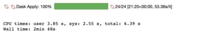
We see a reduction of CPU time by 99.3%. Though one must remember to use these methods carefully since they will not serialize the output therefore using them via grouping can be a good means to leverage this capability.

5. MASE as a metric

 
 
With the rise of using Machine Learning and Deep Learning approaches for time series forecasting, it is essential to use a metric NOT just based on the distance between predicted and actual value. A metric for a forecasting model should use errors from the temporal trend as well to evaluate how well a model is performing instead of just point in time error estimates. Enter Mean Absolute Scaled Error! This metric that takes into account the error we would get if we used a random walk approach where last timestamp’s value would be the forecast for the next timestamp. It compares the error from the model to the error from the naive forecast.

def MASE(y_train, y_test, pred): 
  
    naive_error = np.sum(np.abs(np.diff(y_train)))/(len(y_train)-1)        
    model_error = np.mean(np.abs(y_test - pred))return model_error/naive_error

If MASE > 1 then the model is performing worse than a random walk. The closer the MASE is to 0, the better the forecasting model.

In this article, we went through some of the tricks I often use to make my life easier as a Data Scientist. Comment to share some of your tips! I would love to learn more about tricks that other Data Scientists use in their work.

This is also my first Medium article and I feel like I am talking to nothingness so if you have any feedback to share then please feel free to critique and reach out :)

Thanks to Anne Bonner.

 
Bio: Shree Vandana is a Data Scientist at Amazon, has a Master of Science in Data Science from the University of Rochester, and is excited about all things data and machine learning!

Original. Reposted with permission.

Related:

• How to Select an Initial Model for your Data Science Problem
• ROC Curve Explained
• How to Query Your Pandas Dataframe