Hands-on Reinforcement Learning Course Part 3: SARSA

 

Welcome to my reinforcement learning course ❤️

This is part 3 of my hands-on course on reinforcement learning, which takes you from zero to HERO ????‍♂️. Today we will learn about SARSA, a powerful RL algorithm.

We are still at the beginning of the journey, solving relatively easy problems.

In part 2 we implemented discrete Q-learning to train an agent in the Taxi-v3 environment.

Today, we are going one step further to solve the MountainCar environment ???? using SARSA algorithm.

Let’s help this poor car win the battle against gravity!

All the code for this lesson is in this Github repo. Git clone it to follow along with today’s problem.

 

1. The Mountain car problem ????

 
The Mountain Car problem is an environment where gravity exists (what a surprise) and the goal is to help a poor car win the battle against it.

The car needs to escape the valley where it got stuck. The car’s engine is not powerful enough to climb up the mountain in a single pass, so the only way to make it is to drive back and forth and build sufficient momentum.

Let’s see it in action:

Sarsa Agent in action!

 

The video you just saw corresponds to the SarsaAgent we will build today.

Fun, isn’t it?

You might be wondering.

This looks cool, but why did you choose this problem in the first place?

Why this problem?

The philosophy of this course is to progressively add complexity. Step-by-step.

Today’s environment represents a small but relevant increase in complexity when compared to theTaxi-v3 environment from part 2.

But, what exactly is harder here?

As we saw in part 2, the difficulty of a reinforcement learning problem is directly related to the size of

• the action space: how many actions can the agent choose from at each step?
• the state space: in how many different environment configurations can the agent find itself?

For small environments with a finite (and small) number of actions and states, we have strong guarantees that algorithms like Q-learning will work well. These are called tabular or discrete environments.

Q-functions are essentially matrices with as many rows as states and columns as actions. In these small worlds, our agents can easily explore the states and build effective policies. As the state space and (especially) the action space becomes larger, the RL problem becomes harder to solve.

Today’s environment is NOT tabular. However, we will use a discretization “trick” to transform it into a tabular one, and then solve it.

Let’s first get familiar with the environment!

 

2. Environment, actions, states, rewards

 
???????? notebooks/00_environment.ipynb

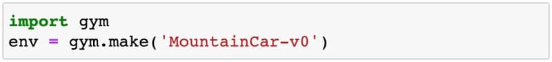
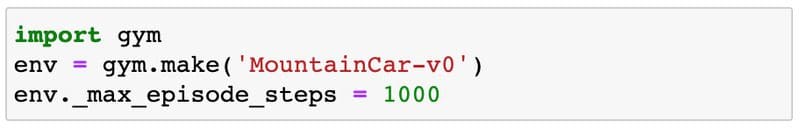
Let’s load the environment:

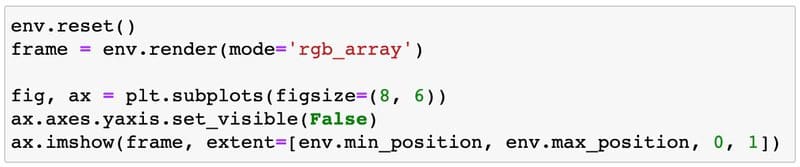
And plot one frame:

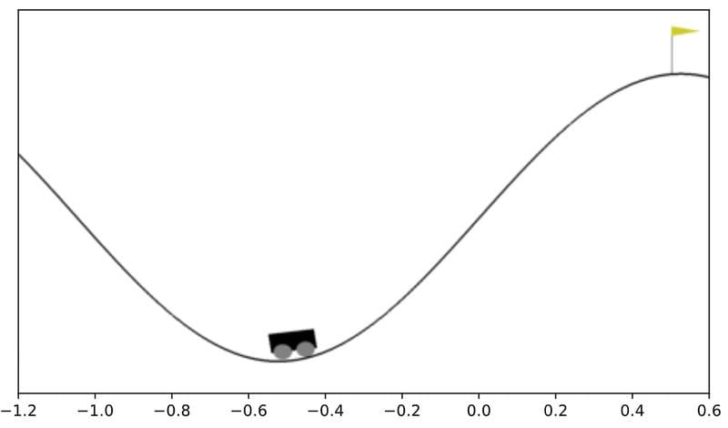
Two numbers determine the state of the car:

• Its position, which ranges from -1.2 to 0.6
• Its speed, which ranges from -0.07 to 0.07.

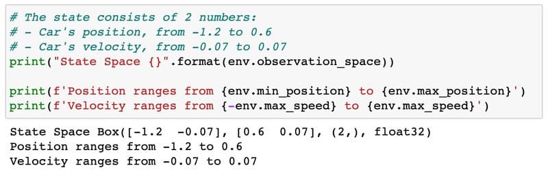
The state is given by 2 continuous numbers. This is a remarkable difference with respect to the Taxi-v3 environment from part 2. We will later see how to handle this.

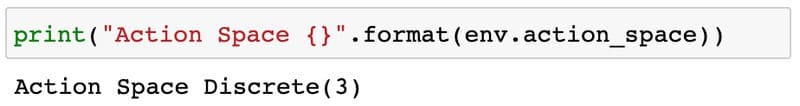
What are the actions?

There are 3 possible actions:

• 0 Accelerate to the left
• 1 Do nothing
• 2 Accelerate to the right

And the rewards?

• A reward of -1 is awarded if the position of the car is less than 0.5.
• The episode ends once the car’s position is above 0.5, or the max number of steps has been reached: n_steps >= env._max_episode_steps

A default negative reward of -1 encourages the car to escape the valley as fast as possible.

In general, I recommend you check Open AI Gym environments’ implementations directly in Github to understand states, actions, and rewards.

The code is well documented and can help you quickly understand everything you need to start working on your RL agents. MountainCar ‘s implementation is here, for example.

Good. We got familiar with the environment.

Let’s build a baseline agent for this problem!

 

3. Random agent baseline ????????

 
???????? notebooks/01_random_agent_baseline.ipynb

Reinforcement learning problems can grow in complexity pretty easily. Well-structured code is your best ally to keep complexity under control.

Today we are going to level up our Python skills and use a BaseAgent class for all our agents. From this BaseAgent class, we will derive our RandomAgent and SarsaAgent classes.

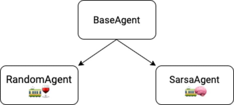
BaseAgent is an abstract class we define in src/base_agent.py

It has 4 methods.

Two of its methods are abstract, which means we are forced to implement them when we derived our RandomAgent and SarsaAgent from the BaseAgent:

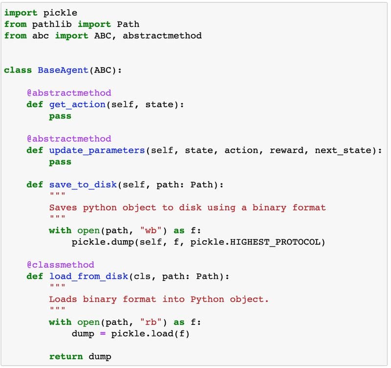
• get_action(self, state) → returns the action to perform, depending on the state.
• update_parameters(self, state, action, reward, next_state) → adjusts agent parameters using experience. Here we will implement the SARSA formula.

The other two methods let us save/load the trained agent to/from the disk.

• save_to_disk(self, path)
• load_from_disk(cls, path)

As we start implementing more complex models and training times increase, it is going to be a great idea to save checkpoints during training.

Here is the complete code for our BaseAgent class:

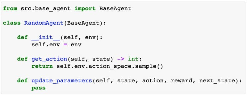
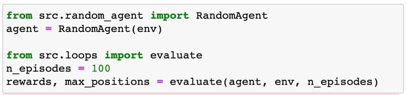
From this BaseAgent class, we can define the RandomAgent as follows:

Let’s evaluate this RandomAgent over n_episodes = 100 to see how well it fares:

And the success rate of our RandomAgentis…

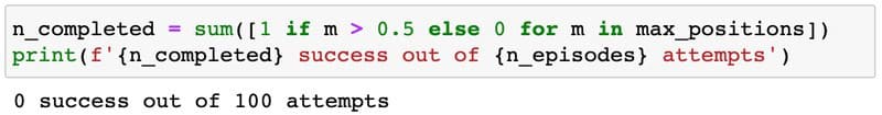
0% ????…

We can see how far the agent got in each episode with the following histogram:

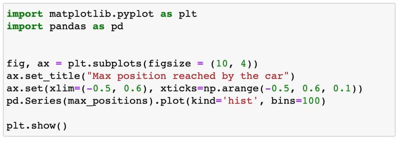
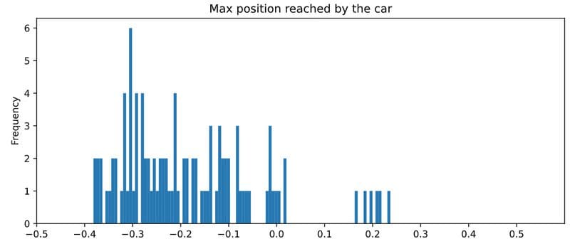
In these 100 runs our RandomAgentdid not cross the 0.5 mark. Not a single time.

When you run this code on your local machine you will get slightly different results, but the percentage of completed episodes above 0.5 will be very far from 100% in any case.

You can watch our miserable RandomAgent in action using the nice show_video function in src/viz.py

A random agent is not enough to solve this environment.

Let’s try something smarter ????…

 

4. SARSA agent ????????

 
???????? notebooks/02_sarsa_agent.ipynb

SARSA (by Rummery and Niranjan) is an algorithm to train reinforcement learning agents by learning the optimal q-value function.

It was published in 1994, two years after Q-learning (by Chris Walkins and Peter Dayan).

SARSA stands for State Action Reward State Action.

Both SARSA and Q-learning exploit the Bellman equation to iteratively find better approximations to the optimal q-value function Q*(s, a)

If you remember from part 2, the update formula for Q-learning is

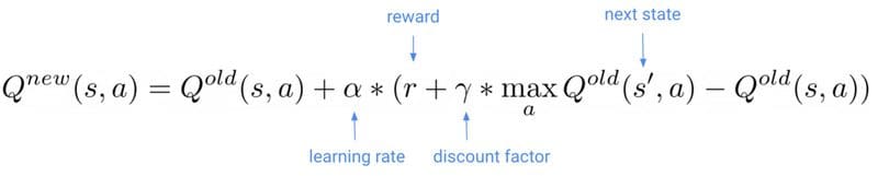
This formula is a way to compute a new estimate of the q-value that is closer to

This quantity is a target ???? we want to correct our old estimate towards. It’s an estimation of the optimal q-value we should aim at, that changes as we train the agent and our q-value matrix gets updated.

Reinforcement learning problems often look like supervised ML problems with moving targets ???? ????

SARSA has a similar update formula but with a different target

SARSA’s target

depends also on the action a’ the agent will take in the next state s’. This is the final A in SARSA’s name.

If you explore enough the state space and update your q-matrices with SARSA you will get to an optimal policy. Great!

You might be thinking…

Q-learning and SARSA look almost identical to me. What are the differences? ????

On-policy vs Off-policy algorithms

There is one key difference between SARSA and Q-learning:

???? SARSA’s update depends on the next action a’, and hence on the current policy. As you train and the q-value (and associated policy) get updated the new policy might produce a different next action a’’ for the same state s’.

You cannot use past experiences (s, a, r, s’, a’) to improve your estimates. Instead, you use each experience once to update the q-values and then throw it away.

Because of this, SARSA is called an on-policy method

???? In Q-learning, the update formula does not depend on the next action a’, but only on (s, a, r, s’). You can reuse past experiences (s, a, r, s’), collected with an old version of the policy, to improve the q-values of the current policy.Q-learning is an off-policy method.

Off-policy methods need less experience to learn than on-policy methods because you can re-use past experiences several times to improve your estimates. They are more sample efficient.

However, off-policy methods have issues converging to the optimal q-value function Q*(s, a) when the state, action spaces grow. They can be tricky and unstable.

We will encounter these trade-offs later in the course when we enter the Deep RL territory ????.

Going back to our problem…

In the MountainCar environment, the state is not discrete, but a pair of continuous values (position s1, velocity s2).

Continuous essentially means infinite possible values in this context. If there are infinite possible states, it is impossible to visit them all to guarantee that SARSA will converge.

To fix that we can use a trick.

Let’s discretize the state vector into a finite set of values. Essentially, we are not changing the environment, but the representation of the state the agent uses to choose its actions.

Our SarsaAgent discretizes the state (s1, s2) from continuous to discrete, by rounding the position [-1.2 … 0.6]to the closest 0.1 mark, and the velocity [-0.07 ...0.07] to the closest 0.01 mark.

This function does exactly that, translate continuous into discrete states:

Once the agent uses a discretized state, we can use the SARSA update formula from above, and as we keep on iterating we will get closer to an optimal q-value.

This is the whole implementation of the SarsaAgent

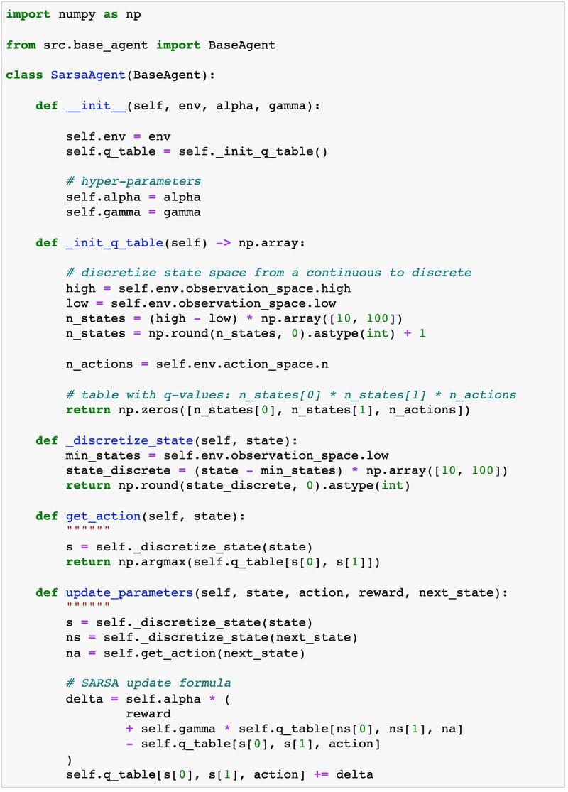
Note ???? that the q-value function is a matrix with 3 dimensions: 2 for the state (position, velocity) and 1 for the action.

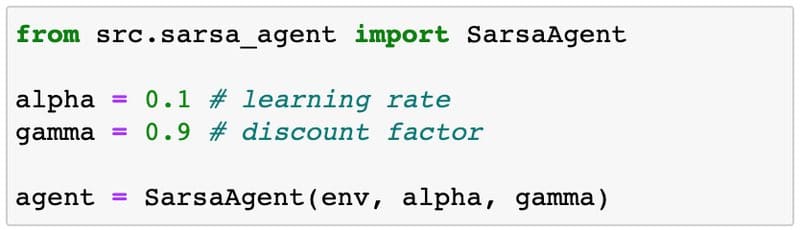
Let’s choose sensible hyper-parameters and train thisSarsaAgent for n_episodes = 10,000

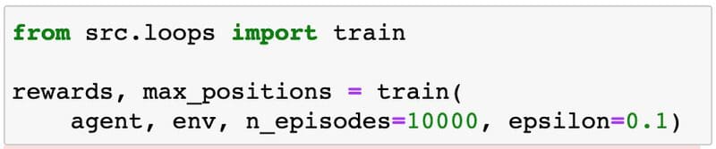
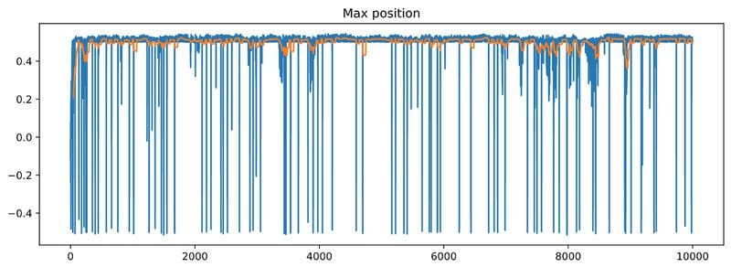
Let’s plot rewards and max_positions (blue lines) with their 50-episode moving averages (orange lines)

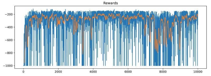
Super! It looks like our SarsaAgent is learning.

Here you can see it in action:

If you observe the max_position chart above you will realize that the car occasionally fails to climb the mountain.

How often does that happen? Let’s evaluate the agent on 1,000 random episodes:

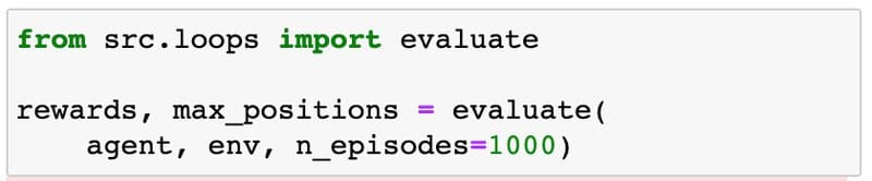
And compute the success rate:

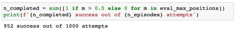
95.2% is pretty good. Still, not perfect. Put a pin on this, we will come back later in the course.

Note: When you run this code on your end you will get slightly different results, but I bet you won’t get a 100% performance.

Great job! We implemented a SarsaAgent that learns ????

It is a good moment to take a pause…

 

5. Take a pause and breath ⏸????

 
???????? notebooks/03_momentum_agent_baseline.ipynb

What if I told you that the MountainCar environment has a much simpler solution…

that works 100% of the time? ????

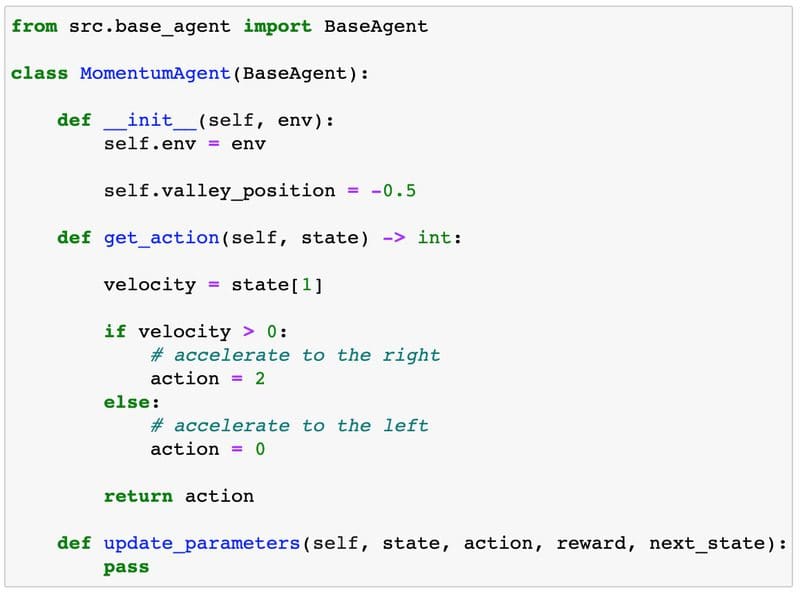
The best policy to follow is simple.

Just follow the momentum:

• accelerate right, when the car is moving to the right velocity > 0
• accelerate left, when the car is moving to the left velocity <= 0

Visually this policy looks like this:

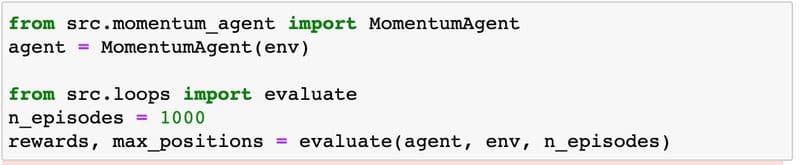
This is how you write this MomentumAgent in Python:

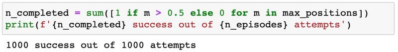
You can double-check it completes every single episode. 100% success rate.

If you plot the trainedSarsaAgent ‘s policy, on the other hand, you will see something like this:

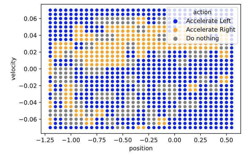
Which has a 50% overlap with the perfect MomentumAgent policy

This means our SarsaAgent is right only 50% of the time.

This is interesting…

Why is the SarsaAgent wrong so often but still achieves good performance?

This is because the MountainCar is still a small environment, so taking wrong decisions 50% of the time is not so critical. For larger problems, being wrong so often is not enough to build intelligent agents.

Would you buy a self-driving car that is right 95% of the time? ????

Also, do you remember the discretization trick we used to apply SARSA? That was a trick that helped us a lot but also introduced an error/bias to our solution.

Why don’t we increase the resolution of the discretization for the state and velocity, to get a better solution?

The problem of doing this is the exponential growth in the number of states, also called the curse of dimensionality. As you increase the resolution of each state component, the total number of states grows exponentially. The state-space grows too fast for the SARSA agent to converge to the optimal policy in a reasonable amount of time.

Ok, but are there any other RL algorithms that can solve this problem perfectly?

Yes, there are. And we will cover them in upcoming lectures. In general, there is no one-size-fits-all when it comes to RL algorithms, so you need to try several of them for your problem to see what works best.

In the MountainCar environment, the perfect policy looks so simple that we can try to learn it directly, without the need to compute complicated q-value matrices. A policy optimization method will probably work best.

But we are not going to do this today. If you want to solve this environment perfectly using RL, follow along with the course.

Enjoy what you’ve accomplished today.

Who is having fun?

 

6. Recap ✨

 
Wow! We covered a lot of things today.

These are the 5 takeaways:

• SARSA is an on-policy algorithm you can use in tabular environments.
• Small continuous environments can be treated as tabular, using a discretization of the state, and then solved with tabular SARSA or tabular Q-learning.
• Larger environments cannot be discretized and solved because of the curse of dimensionality.
• For more complex environments than MountainCarwe will need more advanced RL solutions.
• Sometimes RL is not the best solution. Keep that in mind when you try to solve the problems you care about. Do not marry your tools (in this case RL), instead focus on finding a good solution. Do not miss the forest for the trees ????????????.

 

7. Homework ????

 
???????? notebooks/04_homework.ipynb

This is what I want you to do:

1. Git clone the repo to your local machine.
2. Setup the environment for this lesson 02_mountain_car
3. Open 02_mountain_car/notebooks/04_homework.ipynband try completing the 2 challenges.

In the first challenge, I ask you to tune the SARSA hyper-parameters alpha (learning rate) and gamma (discount factor) to speed up training. You can get inspiration from part 2.

In the second challenge, try to increase the resolution of the discretization and learn the q-value function with tabular SARSA. As we did today.

Let me know if you build an agent that achieves 99% performance.

 

8. What’s next? ❤️

 
In the next lesson, we are going to enter a territory where Reinforcement Learning and Supervised Machine Learning intersect ????.

It is going to be pretty cool, I promise.

Until then,

Enjoy one more day on this amazing planet called Earth ????

Love ❤️

And keep on learning ????

If you like the course, please share it with friends and colleagues.

You can reach me under plabartabajo@gmail.com . I would love to connect.

See you soon!

 
 
Bio: Pau Labarta Bajo (@paulabartabajo_) is a mathematician and AI/ML freelancer and speaker, with over 10 years of experience crunching numbers and models for different problems, including financial trading, mobile gaming, online shopping, and healthcare.

Original. Reposted with permission.