Hands-On with Supervised Learning: Linear Regression
If you're looking for a hands-on experience with a detailed yet beginner-friendly tutorial on implementing Linear Regression using Scikit-learn, you're in for an engaging journey.
Image by Author
Basic Overview
Linear regression is the fundamental supervised machine learning algorithm for predicting the continuous target variables based on the input features. As the name suggests it assumes that the relationship between the dependant and independent variable is linear. So if we try to plot the dependent variable Y against the independent variable X, we will obtain a straight line. The equation of this line can be represented by:

Where,
- Y Predicted output.
- X = Input feature or feature matrix in multiple linear regression
- b0 = Intercept (where the line crosses the Y-axis).
- b1 = Slope or coefficient that determines the line's steepness.
The central idea in linear regression revolves around finding the best-fit line for our data points so that the error between the actual and predicted values is minimal. It does so by estimating the values of b0 and b1. We then utilize this line for making predictions.
Implementation Using Scikit-Learn
You now understand the theory behind linear regression but to further solidify our understanding, let's build a simple linear regression model using Scikit-learn, a popular machine learning library in Python. Please follow along for a better understanding.
1. Import Necessary Libraries
First, you will need to import the required libraries.
import os
import pandas as pd
import numpy as np
import matplotlib.pyplot as plt
from sklearn.linear_model import LinearRegression
from sklearn.preprocessing import StandardScaler
from sklearn.metrics import mean_squared_error
2. Analyzing the Dataset
You can find the dataset here. It contains separate CSV files for training and testing. Let’s display our dataset and analyze it before proceeding forward.
# Load the training and test datasets from CSV files
train = pd.read_csv('train.csv')
test = pd.read_csv('test.csv')

# Display the first few rows of the training dataset to understand its structure
print(train.head())
Output:
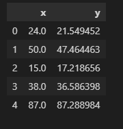
train.head()
The dataset contains 2 variables and we want to predict y based on the value x.
# Check information about the training and test datasets, such as data types and missing values
print(train.info())
print(test.info())
Output:
RangeIndex: 700 entries, 0 to 699
Data columns (total 2 columns):
 #   Column  Non-Null Count  Dtype
---  ------  --------------  -----
 0   x       700 non-null    float64
 1   y       699 non-null    float64
dtypes: float64(2)
memory usage: 11.1 KB


RangeIndex: 300 entries, 0 to 299
Data columns (total 2 columns):
 #   Column  Non-Null Count  Dtype
---  ------  --------------  -----
 0   x       300 non-null    int64
 1   y       300 non-null    float64
dtypes: float64(1), int64(1)
memory usage: 4.8 KB
The above output shows that we have a missing value in the training dataset that can be removed by the following command:
train = train.dropna()
Also, check if your dataset contains any duplicates and remove them before feeding it into your model.
duplicates_exist = train.duplicated().any()
print(duplicates_exist)
Output:
False
2. Preprocessing the Dataset
Now, prepare the training and testing data and target by the following code:
#Extracting x and y columns for train and test dataset
X_train = train['x']
y_train = train['y']
X_test = test['x']
y_test = test['y']
print(X_train.shape)
print(X_test.shape)
Output:
(699, )
(300, )
You can see that we have a one-dimensional array. While you could technically use one-dimensional arrays with some machine learning models, it's not the most common practice, and it may lead to unexpected behavior. So, we will reshape the above to (699,1) and (300,1) to explicitly specify that we have one label per data point.
X_train = X_train.values.reshape(-1, 1)
X_test = X_test.values.reshape(-1,1)
When the features are on different scales, some may dominate the model's learning process, leading to incorrect or suboptimal results. For this purpose, we perform the standardization so that our features have a mean of 0 and a standard deviation of 1.
Before:
print(X_train.min(),X_train.max())
Output:
(0.0, 100.0)
Standardization:
scaler = StandardScaler()
scaler.fit(X_train)
X_train = scaler.transform(X_train)
X_test = scaler.transform(X_test)
print((X_train.min(),X_train.max())
Output:
(-1.72857469859145, 1.7275858114641094)
We are now done with the essential data preprocessing steps, and our data is ready for training purposes.
4. Visualizing the Dataset
It's important to first visualize the relationship between our target variable and feature. You can do this by making a scatter plot:
# Create a scatter plot
plt.scatter(X_train, y_train)
plt.xlabel('X')
plt.ylabel('Y')
plt.title('Scatter Plot of Train Data')
plt.grid(True)  # Enable grid
plt.show()
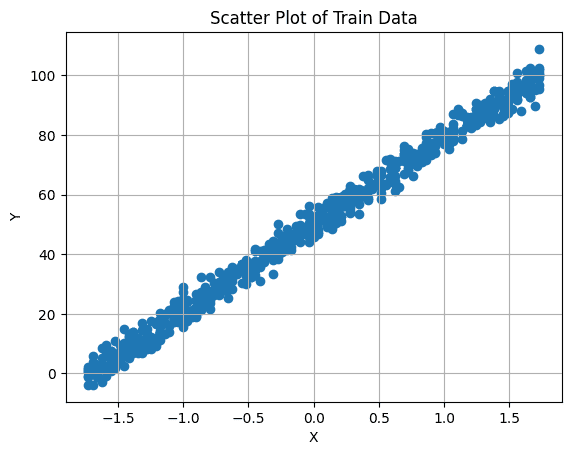
Image by Author
5. Create and Train the Model
We will now create an instance of the Linear Regression model using Scikit Learn and try to fit it into our training dataset. It finds the coefficients (slopes) of the linear equation that best fits your data. This line is then used to make the predictions. Code for this step is as follows:
# Create a Linear Regression model
model = LinearRegression()

# Fit the model to the training data
model.fit(X_train, y_train)

# Use the trained model to predict the target values for the test data
predictions = model.predict(X_test)

# Calculate the mean squared error (MSE) as the evaluation metric to assess model performance
mse = mean_squared_error(y_test, predictions)
print(f'Mean squared error is: {mse:.4f}')
Output:
Mean squared error is: 9.4329
6. Visualize the Regression Line
We can plot our regression line using the following command:
# Plot the regression line
plt.plot(X_test, predictions, color='red', linewidth=2, label='Regression Line')

plt.xlabel('X')
plt.ylabel('Y')
plt.title('Linear Regression Model')
plt.legend()
plt.grid(True)
plt.show()
Output:
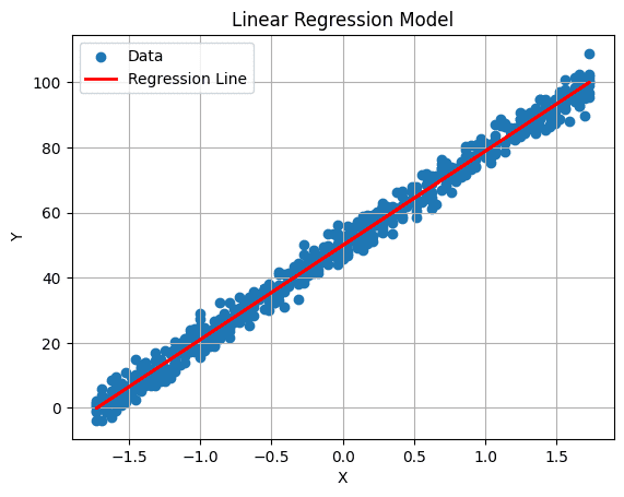
Image by Author
Conclusion
That's a wrap! You've now successfully implemented a fundamental Linear Regression model using Scikit-learn. The skills you've acquired here can be extended to tackle complex datasets with more features. It's a challenge worth exploring in your free time, opening doors to the exciting world of data-driven problem-solving and innovation.
Kanwal Mehreen is an aspiring software developer with a keen interest in data science and applications of AI in medicine. Kanwal was selected as the Google Generation Scholar 2022 for the APAC region. Kanwal loves to share technical knowledge by writing articles on trending topics, and is passionate about improving the representation of women in tech industry.