Weak Supervision Modeling, Explained
This article dives into weak supervision modeling and truly understanding the label model.
What is Weak Supervision?
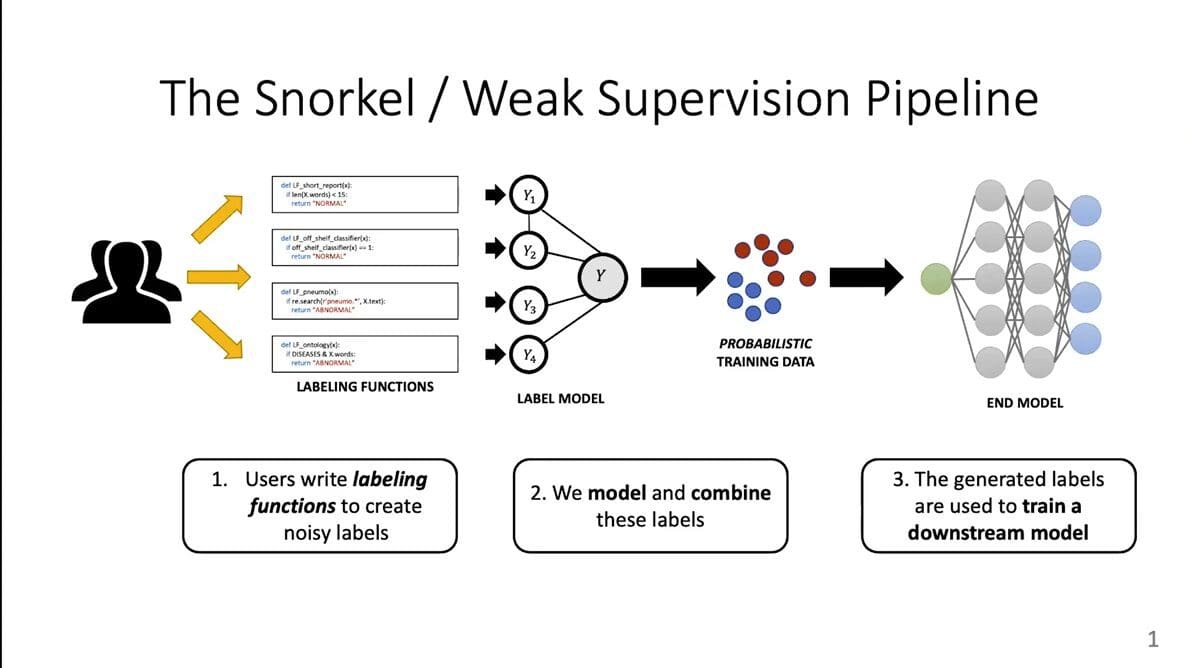
Weak supervision is a way to obtain labels for training data points for a machine learning model programmatically, by writing labeling functions. These functions label your data much faster and more efficiently than manual labeling, but they also create “noisy” labels, which you then need to model and combine in order to generate the labels that you will later use to train your downstream model. In other words, there is little-to-no actual hand labeling being done by a human, instead, the labeling is done programmatically and then “de-noised” via a label model.
In this post, we will be focusing primarily on the middle section of this pipeline: the label model itself. This is the object used to model and combine the noisy labels.
Creating the Label Model in Weak Supervision
One way to think about de-noising is to combine noisy labels—but all of the labeling functions aren’t necessarily equally reliable! When you generate a label model, then, you are asking: how do you know which of the noisy labels produced by the programmatic labeling function are reliable? Essentially, you need to figure out which ones you should throw out or not, and then how to use them. By doing that, you can determine the “best guess” of what the actual label should be, and that provides you with an automatically constructed data set. You then train your final model using those labels.

What is the intuition behind a label model? To use a simplistic analogy, imagine a courtroom full of witnesses. We usually refer to the “true” label for a data point as being a latent, unobserved variable, and that is exactly what happens in court. You don't know whether the defendant actually committed the crime or not. So, you have to use some alternative forms of learning the truth. In this very simplistic analogy, each witness says, “I think the defendant committed the crime,” or, “I do not think the defendant committed the crime.”
The witnesses are a lot like our labeling functions. The variable of whether the defendant committed the crime or not is kind of like a “+1; -1” label for our case. One witness is +1, one witness is +1, one witness is -1, and so on. From there, the easiest thing to do is to go with what the majority of witnesses say, and this is exactly what the majority-vote aspect of the label model is doing as well. It says, “the majority of the labeling function said +1, so this data point is a +1.” You can get a lot from doing this. But there are some downsides.
Accuracies and Correlations
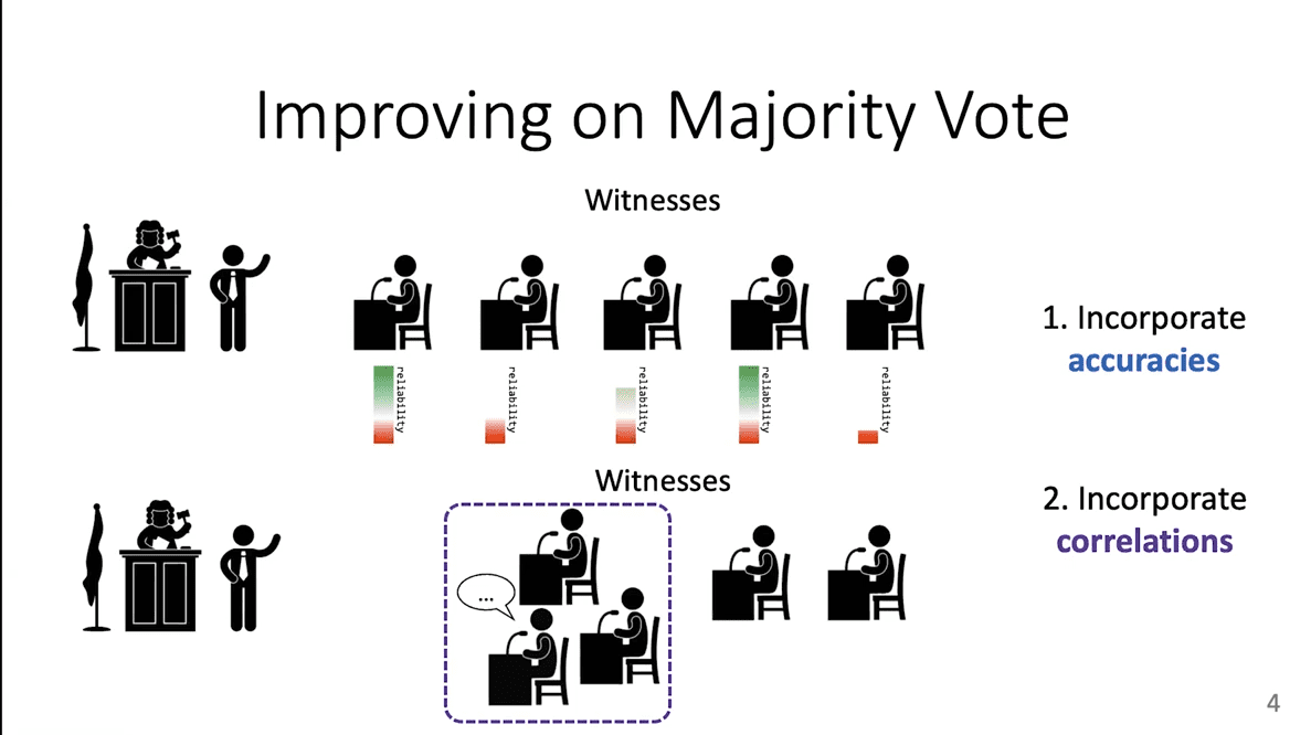
There are two major downsides to majority vote, for our purposes. One is that not all witnesses are equally reliable. You don't want to simply throw out the witnesses that are not as reliable, but you do want to assign them different weights. The hard part is that you don't know for sure which witnesses are reliable or unreliable. You have to figure it out on your own. We call this process finding “accuracies.” We want our label model to incorporate the accuracies of the labeling function.
The second downside is something called correlations or “cliques.” Imagine if three of the witnesses cooperated and talked together before the trial began. You would not want to trust them as much as you might three independent witnesses, because once they coordinated, they may have come to change their minds and agree on a single view. Ideally, you want to then down-weight these “cliques” of witnesses.
Majority vote cannot help us with either of these problems. It simply gives equal weight to everybody, reliable or unreliable, and it gives equal weight to everybody even if they form a clique. But you want to include accuracies and correlations in your label model, which means we will have to learn about them.
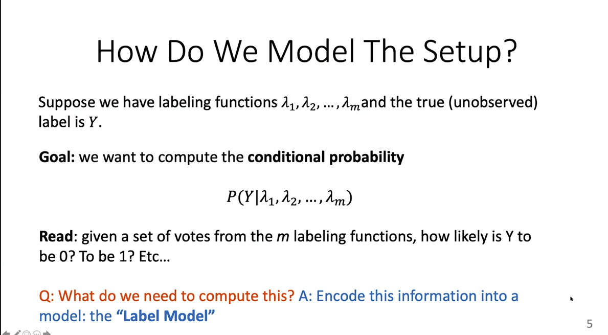
From this point forward, the math we will use is this notation: “lambda 1,” “lambda 2,” through “lambda n.” These are your labeling functions. They're random variables, and they take on values like -1 or +1. Then, there is the true but unobserved label “Y.” You don’t get to see it, but it's there.
Very concretely, your goal is to compute this conditional probability P(Y) given ? 1 ? 2 through ? n. It is the probability of the label, having known that we have this information from the labeling functions. In other words: what is the probability, given all of the noisy labels that you have, that Y has value 0 or 1 or 2, and so on.
This is already a big improvement over majority vote, because you don't have to just say, “I think it is +1.” Instead, you can say, “I think it is a probability of 0.6 of being +1 and 0.3 of being -1,” and so on. That is already a lot more useful for training your eventual model. But you still don’t know enough to compute your conditional probability. In order to do that, you need to encode all of your information into what we call a label model.
This is what a label model really is: it is all of the information that you need to compute these conditional probabilities, which then tell you, given the labeling functions’ output, what is the probability of every possible value of the true label, Y?
What’s a Probabilistic Model?
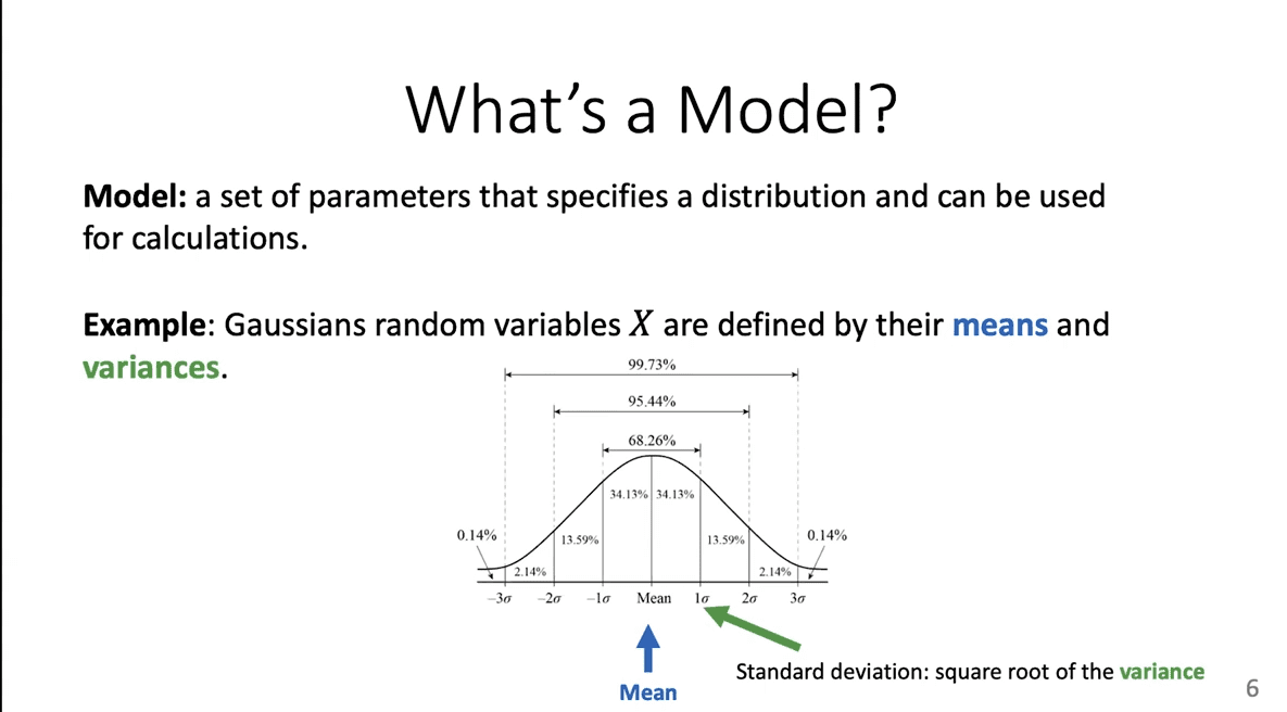
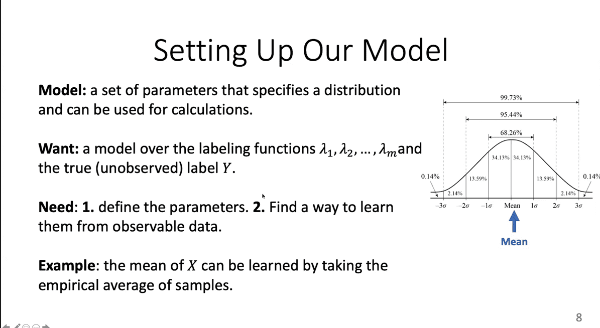
In order to compute your conditional probability, you need a probabilistic model. A probabilistic model is a set of parameters that can fully specify some distribution that you can use for calculations.
A really simple example is Gaussian random variables. You can think of one as a model just by itself if you know the mean and the variance. So, ifitell you the mean and the variance, you can say, for example, “the probability that X equals 3.7 is ___; the probability that X is between -2 and 16 is ___,” and so on.
For your label model, you want to define similar things. You want to find: what are the parameters that are sufficient for you to compute the conditional probabilities for the true label, given the values of the labeling function.
Random Variables
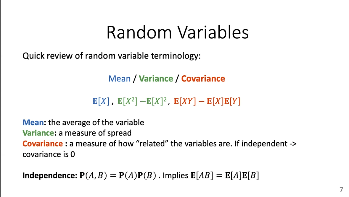
Let’s pause here and review a quick primer on random variables.
In the classic image of the bell curve above, the mean is in the middle. That is the expectation of X. The variance is the measure of the spread—how far away you are from the mean, on average.
The covariance between two variables is a measure of how related two variables are. When variables are independent, meaning they have no information about one another, their covariance is 0. You can already think of this as defining an accuracy. We want to know the covariance between one labeling function and the true label, Y. If a given labeling function is really bad at guessing the Y, the covariance between these two things will be 0.
Finally, there is the independence property: A and B are independent if, and only if, P(AB) is P(A) times P(B). This implies that the expectations for these two things you can write the product as the product of the expectations.
Setting Up Your Model
Now, let’s set up your actual label model.
On a data-centric AI approach, the label model involves all of these variables, the labeling functions in the true label, Y, and then of course you need to learn these parameters from data, because you don't know them a priori. In this Gaussian case, for example, you could compute the mean by simply taking a lot of samples, adding them up, and normalizing, dividing by how many samples you saw. You can think of a coin flip in the same way. If the probability of heads is P, you can estimate P by flipping a coin 10,000 times, seeing how many heads come up, and dividing by 10,000. That's an empirical estimate of P. For our purposes, you have to do a very similar procedure.
A brief recap: You want to improve on simple majority vote by integrating the accuracies of the labeling functions as well as their correlations, or “cliques.” To do so, you have to introduce some probabilistic model over the labeling functions in the true label. You need to learn what the appropriate parameters are that encode all this information. You need to have a way to learn these parameters. And then you need to find what calculation is going to give us that conditional probability.
In other words: What is the probability of the true label, Y, given what we saw from the wavelength functions? You won't ever get to see Y. That's the whole idea behind weak supervision. You will only see samples from the labeling functions, and that's the information you get to use.
Now, let's specify what these parameters are actually going to be.
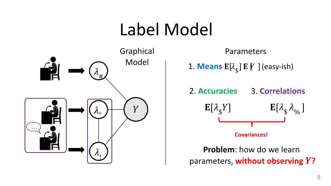
Obviously, you want things like the means, so the expectations of each of these labeling functions, ? i, is also the expectation of Y. These things are not very difficult to estimate. To find the expectation of ? i, look at all of the outputs for the labeling function, and then see how often it votes +1, how often it votes -1, divided by the total, and that gives you the mean.
The expectation of Y is harder, because you don't get to see the true labels, but you can get this too if you have, say, a dev set. You can get an estimate of the class balance from a dev set, and there are other ways to do this as well.
These are the means, and if you recall from the Gaussian example above, the means and the variances give you everything you need. It's going to be the same thing here. The variances (or covariances) are going to be these accuracies and these correlations. The expectation of ?itimes Y, and then the expectations of this product ? i comes ? J.
Assume we're talking about binary variables, here. So they are all either +1 or -1. Of course, this is just for illustration—we can do slightly more sophisticated things if we have multiclass label values. If your ? i—your labeling function—is really accurate, then it's going to always agree with Y. So when Y is 1, it's going to be 1. When Y is -1, it's going to be -1. This product will always be 1, because 1 times 1 is 1 and -1 times -1 is also 1. This expectation is going to be close to 1 all of the time. If your labeling function is really inaccurate, you are going to be close to 0 all of the time. This kind of parameter will tell us how accurate the actual labeling functions are, and that's why we can justify this accuracy terminology.
Correlations are the same. How often do labeling functions agree with each other or how often do they disagree with each other? Then in the cases where there are these correlations you are going to get one correlation as well. This gives you all of the parameters of the model. Just like the Gaussian example, you have these means, and you have the covariance instead of the variance. If you know these, you have enough information to compute those conditional probabilities. This is the whole goal for the label model, and everything else follows from there.
This is all much more difficult to do when compared to the coin flip example. Normally, if you were computing a mean, you would view a lot of samples and just find their average. But you don't know what Y is in this case, so you can't just take samples of ?itimes Y. That's the hard part about weak supervision. You don't know the true label, so you cannot easily compute these kinds of empirical expectations. That's the only real trick that you need to use here for the label model: a way to get access to this information without actually knowing what Y is.
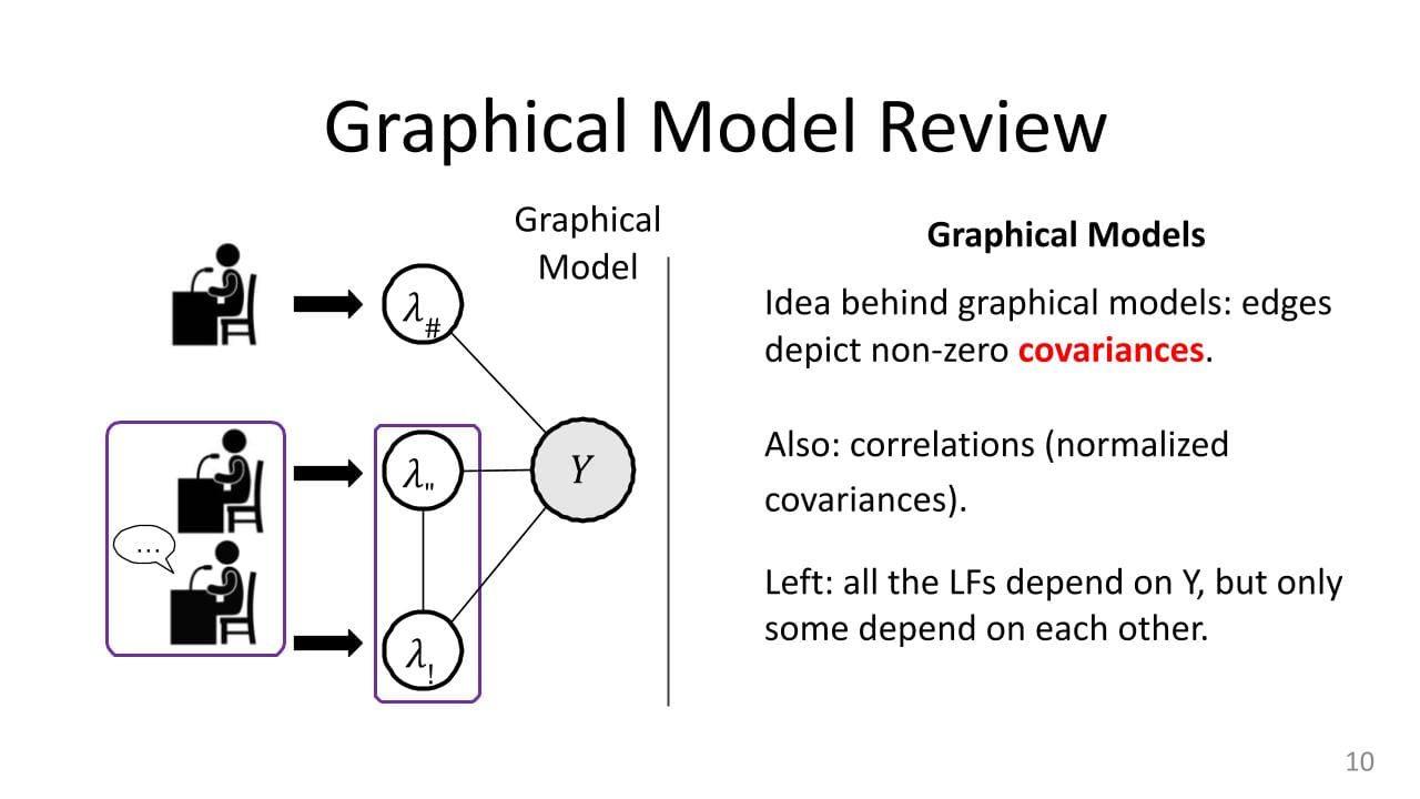
In this graphical model, there is a node for every random variable. The edges tell you something about correlations or covariances. There is a real technical explanation for what exactly they mean, but very roughly, if there is an edge between things you can think of them as correlated. If there is no edge between a pair of nodes, you can think of them as having some independence between them. Sometimes, you have to do something to the variables to find that independence, but that is the basic idea. In this setup, the labeling functions are always connected to the true label. If they were not, then there would be no relationship between the labeling function value and the label. You would have a “random guessing” labeling function, which would not be useful. You always have these edges between the actual value of the label and all the labeling functions.
Sometimes you have edges between pairs of labeling functions, and sometimes you don't. When we have that pair, it is in the case of correlations. That was in the courtroom analogy from above, where you have two witnesses talking to each other and coming up with one story. That is something we also want to model, because we do want to down-weight those values. And in fact implicitly when you compute this conditional “P(Y) given ___” probability, you are going to take that into account when you compute it.
How do you learn the parameters. There are two primary methods.
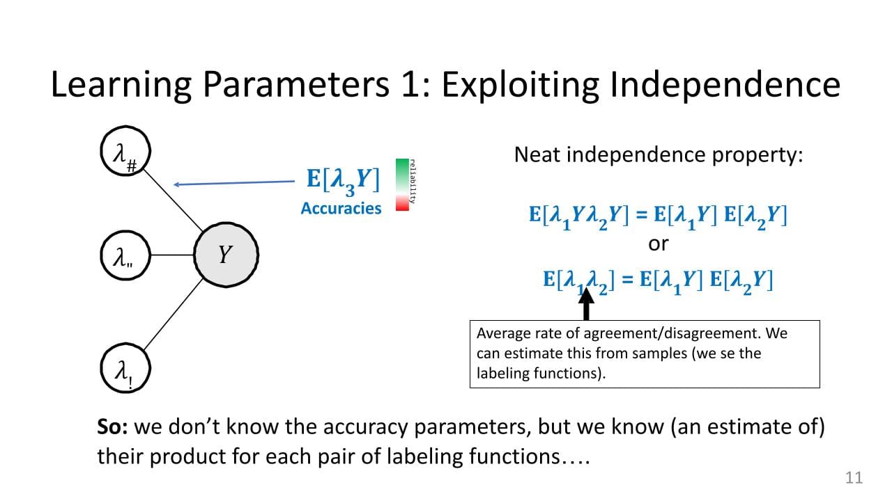
The first is perhaps easiest. The only real parameter we care to know about are the accuracies. To learn it, you want to exploit independence specifically, and that's why, with this graphical model, on the left there are no edges between the labeling functions, only between the labeling functions and the true label.
Again, remember what the accuracy parameters are. There are these expectations of the product of a labeling function, and the bigger they are, the more reliable you can think of a given labeling function. If they were perfectly reliable, you would just use that information for Y. If they are super unreliable, you want to down-weight them.
Let’s look at this really neat property of independence. The labeling functions themselves are not independent of one another, which is good because they are all trying to predict the same thing. If they were independent, they would be terrible. But it turns out that the products of the labeling functions and Y, often are independent. Essentially, the accuracies are independent even though the variables themselves are not independent.
So, what does that mean? If you write this product on the left—this ? 1Y, ? 2Y—you can factorize this product because of independence as the product of two expectations (under some minor assumptions that we won’t get into). It is: expectation of the product is the product of the expectations.
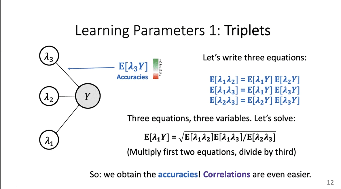
The second method for learning parameters involves using triplets. This Y was +1 or -1. Those are the two possible values. When you multiply ? 1Y ? 2Y, you get ? 1 ? 2Y-squared. But Y-squared is 1, regardless of whether Y is +1 or -1. So this one just goes away, and you end up just seeing ? 1 ? 2's expectation.
So, we are writing the expectation of ? 1Y times ? 2Y, which are these two accuracy parameters. Their product is this correlation parameter thatican actually estimate. This is just the agreement or disagreement on average of a pair of labeling functions. If you look at all the things they have labeled, you can say: “they have the same label 75 percent of the time and they are different 25 percent of the time, and that tells me this expectation of ? 1 ? 2.” In other words, this is observable.idon't really know what the accuracy parameters are for these two labeling functions, butido know that they multiply to be this kind of correlation parameter, which is knowable. We don't know the accuracy parameters but we know a function of the accuracy parameters, which is their product.
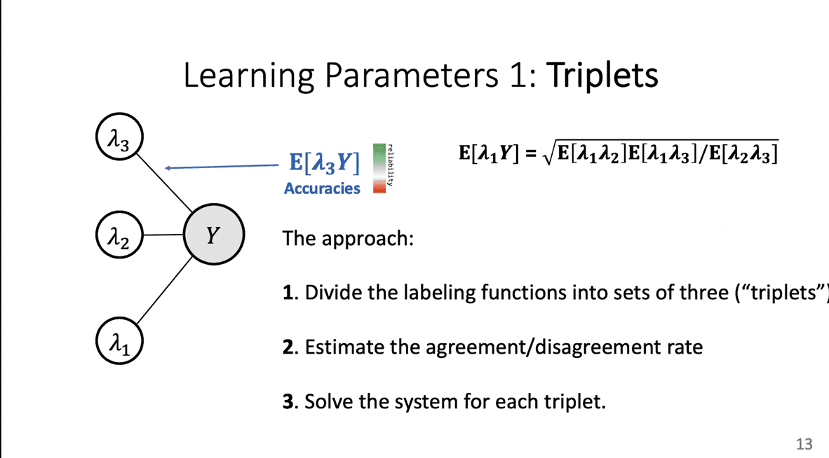
This is actually the key thing that we have to have here. Once we have this, we can do a little system of equations, called triplets. We can write down this exact thing for three labeling functions, just going two at a time. For the three equations above, we just did this exact trick for ? 1 ? 2, and for ? 1 ? 3, then for ? 2 ? 3. We have this independence property between each of these pairs. There are three different pairs and you have three equations and you have three variables. What are the three variables? They are just each of these accuracy parameters. You know the left-hand sides for all these cases, so you can think of this as A times B has some value, A times C has some value, B times C has some value. You know those three values andineed to compute A, B, and C from them. You can solve this.
So, even though you never got to see Y, and even though you cannot directly do a sample average to get this expectation, you have still written it in terms that are observable. You can go into our label matrix and compute these three terms, solve this equation, and get our guess of this product. Thenican do this for every possible labeling function andiwill get all of the accuracies. As for correlation, you can estimate it directly. You simply average them, just like the coin flips. Now we have access to all the accuracies and we are done.
Learning Parameters
- Exploiting Independence
- Triplets
- Covariance Matrix
Where to connect with Fred: Twitter | Website.
Stay in touch with Snorkel AI, follow us on Twitter, LinkedIn, Facebook, Youtube, or Instagram, and if you’re interested in joining the Snorkel team, we’re hiring! Please apply on our careers page.
Frederic Sala is an Assistant Professor in the Computer Sciences Department at the University of Wisconsin-Madison. Fred's research studies the foundations of data-driven systems, with a focus on machine learning systems. Previously, he was a postdoctoral researcher in the Stanford CS department associated with the Stanford InfoLab and Stanford DAWN. He received his Ph.D. in electrical engineering from UCLA in December 2016. He is the recipient of the NSF Graduate Research Fellowship, the outstanding Ph.D. dissertation award from the UCLA Department of Electrical Engineering, and the Edward K. Rice Outstanding Masters Student Award from the UCLA Henry Samueli School of Engineering & Applied Science. He received the B.S.E. degree in Electrical Engineering from the University of Michigan, Ann Arbor.