Predicting Cryptocurrency Prices Using Regression Models
In this article, we explore how to get started with the prediction of cryptocurrency prices using multiple linear regression. The factors investigated include predictions on various time intervals as well as the use of various features in the models such as opening price, high price, low price and volume.

Source: https://unsplash.com/s/photos/cryptocurrency
Introduction
As of March 2022, the cryptocurrency market stands at over $2 trillion [1] but remains incredibly volatile, having previously hit $3 trillion in November 2021. The same volatility is also seen within the individual cryptocurrencies, within the past month alone Etherium and Bitcoin have decreased by over 18% and 19% respectively. The number of new currencies coming onto the market is also increasing, with over 18,000 cryptocurrencies in existence as of March 2022 [2].
This volatility is what makes long-term cryptocurrency predictions more difficult. In this article, we will go through how to get started with cryptocurrency predictions using linear regression models. We will look at predictions over a number of time intervals whilst using various model features, like opening price, high price, low price and volume. The cryptocurrencies looked at in this article include more established players Bitcoin and Etherium as well as those still in fairly early stages namely Polkadot and Stellar.
Method
In this article, we will be using multiple linear regression. Regression models are used to determine the relationship between variables by fitting a line through the data. Simple linear regression is a model used to predict a dependent variable (for instance the closing price of a cryptocurrency) using one independent variable (such as opening price), whereas multiple linear regression takes into account several independent variables.
The data we will be using comes from CoinCodex [3] and provides daily opening, high, low and closing as well as the volume and the market cap. Various combinations of features were experimented with to produce the models with predictions also being made over daily and weekly intervals. The python sklearn package was used to train the models and the R2 value was used as a metric of the accuracy of the model, with 1 indicating a perfect model.
The data used and the models produced have been uploaded to a Layer project and can be downloaded for further use and investigations. All the results and corresponding graphs can also be found in the Layer project. In this article we will discuss sections of the code used to implement the models.The full code can be accessed in this collab notebook.
In order to initialise the project and access the data and models you can run:
import layer
layer.login()
layer.init("predictingCryptoPrices")
The data was uploaded to the Layer project for each of the 4 cryptocurrency datasets (Bitcoing, Ethereum, Polkadot and Stellar) by defining the functions used to read in the data and annotating them with the dataset and resources decorators.
@dataset("bitcoin")
@resources(path="./data")
def getBitcoinData():
    return pd.read_csv("data/bitcoin.csv")

layer.run([getBitcoinData])
You can run the following commands to access the datasets and save them to a pandas dataframe
layer.get_dataset("bitcoin").to_pandas()
layer.get_dataset("ethereum").to_pandas()
layer.get_dataset("polkadot").to_pandas()
layer.get_dataset("stellar").to_pandas()
Predictions
Daily predictions
The first set of multiple regression models were built to predict the prices at daily intervals. The closing price was first predicted using opening, low and high price on that day. Daily prices over the course of 1 year were used with a 75%-25% train-test split. The below function was used to train the model for a given dataset.
def runNoVolumePrediction(dataset):

    # Defining the parameters
    # test_size: proportion of data allocated to testing
    # random_state: ensures the same test-train split each time for reproducibility

    parameters = {
      "test_size": 0.25,
      "random_state": 15,
    }

    # Logging the parameters
    # layer.log(parameters)
    # Loading the dataset from Layer
    df = layer.get_dataset(dataset).to_pandas()
    df.dropna(inplace=True)

    # Dropping columns we won't be using for the predictions of closing price
    dfX = df.drop(["Close", "Date", "Volume", "Market Cap"], axis=1)

    # Getting just the closing price column
    dfy = df["Close"]

    # Test train split (with same random state)
    X_train, X_test, y_train, y_test = train_test_split(dfX, dfy, test_size=parameters["test_size"], random_state=parameters["random_state"])

    # Fitting the multiple linear regression model with the training data
    regressor = LinearRegression()
    regressor.fit(X_train,y_train)

    # Making predictions using the testing data
    predict_y = regressor.predict(X_test)

    # .score returns the coefficient of determination R² of the prediction
    layer.log({"Prediction Score :":regressor.score(X_test,y_test)})

    # Logging the coefficient corresponding to each variable
    coeffs = regressor.coef_
    layer.log({"Opening price coeff":coeffs[0]})
    layer.log({"Low price coeff":coeffs[1]})
    layer.log({"High price coeff":coeffs[2]})

    # Plotting the predicted values against the actual values
    plt.plot(y_test,predict_y, "*")
    plt.ylabel('Predicted closing price')
    plt.xlabel('Actual closing price')
    plt.title("{} closing price prediction".format(dataset))
    plt.show()

    #Logging the plot
    layer.log({"plot":plt})
    return regressor
The function was running with the model decorator to save the model to the Layer project as shown below.
@model(name='bitcoin_prediction')
def bitcoin_prediction():
    return runNoVolumePrediction("bitcoin")

layer.run([bitcoin_prediction])
To access all of the models used in this set of predictions you can run the below code.
layer.get_model("bitcoin_prediction")
layer.get_model("ethereum_prediction")
layer.get_model("polkadot_prediction")
layer.get_model("stellar_prediction")
Table 1 below summarises the R2 statistics for the 4 cryptocurrencies using this model.
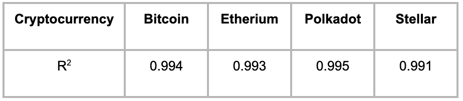
Table 1: Accuracy of predictions of cryptocurrency closing price using opening, low and high prices on that day
The graphs below show the predicted values against the true values for the best and worst-performing currencies Polkadot and Stellar (Figure 1a and 1b).

Figure 1a: Stellar predicted closing price against the true closing price for the day using opening, low and high prices as features
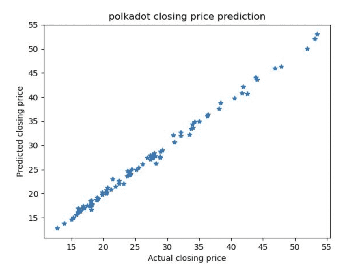
Figure 1b: Polkadot predicted closing price against the true closing price for the day using opening, low and high prices as features
From the graph and the R2 values, we can see that the linear regression model using opening, low and high price is very accurate for all 4 currencies, regardless of their level of maturity.
Next, we investigate whether adding the volume improves the model. The volume corresponds to the total number of trades taking place that day. Interestingly enough after fitting regression models using opening, low and high prices and the volume the results were largely identical. You can access the bitcoin_prediction_with_volume, ethereum_prediction_with_volume, polkadot_prediction_with_volume and stellar_prediction_with_volume models in the Layer project. Further investigation showed, that the coefficient for the volume variable was 0 across the 4 cryptocurrencies. This indicated the volume of trades of a cryptocurrency is not a good predictor of its price on that day.
Weekly predictions
In the next model, we look at predicting the end of week prices using the data from that weeks opening price on a Monday along with the low and high prices that week. For this model data from the past 5 years was used for Bitcoin, Ethereum and Stellar. For Polkadot, which was only launched in 2020, all of the historical data was used.
After downloading the data the low and high prices for each week were calculated and the opening and closing prices for the week were recorded. These datasets can also be accessed on Layer by running:
layer.get_dataset("bitcoin_5Years").to_pandas()
layer.get_dataset("ethereum_5Years").to_pandas()
layer.get_dataset("polkadot_5Years").to_pandas()
layer.get_dataset("stellar_5Years").to_pandas()
Again, a 75%-25% train-test split was used and a multiple linear regression model was fitted using the opening, high and low prices for the week. The models can also be accessed on the Layer project. The R2 metric was again used for comparison with the results shown in Table 2 below.
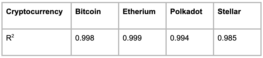
Table 2: Accuracy of predictions of cryptocurrency closing price using opening, low and high prices
The accuracy of the models when predicting with data over the course of a week were slightly worse than when predicting over the course of a day however, the accuracy itself was still very high. Even the worst performing model for the cryptocurrency Stellar achieve and R2 score of 0.985.
Conclusion
Overall, linear regression models using the opening, low and high prices as features perform very well on both daily and weekly intervals. A natural extension of these models would be looking into predicting further into the future, for instance using this weeks data to predict the price next week.
[3] https://coincodex.com/crypto/stellar/historical-data/
Eleonora Shantsila is a full stack software engineer working at an events start up called Lounge, having previously worked as a full stack engineer in Financial Services. Eleonora has a background in Mathematics (BSc from St Andrews University) and Computational Science (MS from Harvard University) and enjoys working on data science projects in their spare time. Feel free to connect on LinkedIn.