Understanding by Implementing: Decision Tree
Learn how a Decision Tree works and implement it in Python.
Image by Author
Many advanced machine learning models such as random forests or gradient boosting algorithms such as XGBoost, CatBoost, or LightGBM (and even autoencoders!) rely on a crucial common ingredient: the decision tree!
Without understanding decision trees, it is impossible to understand any of the aforementioned advanced bagging or gradient-boosting algorithms as well, which is a disgrace for any data scientist! So, let us demystify the inner workings of a decision tree by implementing one in Python.
In this article, you will learn
- why and how a decision tree splits data,
- the information gain, and
- how to implement decision trees in Python using NumPy.
You can find the code on my Github.
The Theory
In order to make predictions, decision trees rely on splitting the dataset into smaller parts in a recursive fashion.
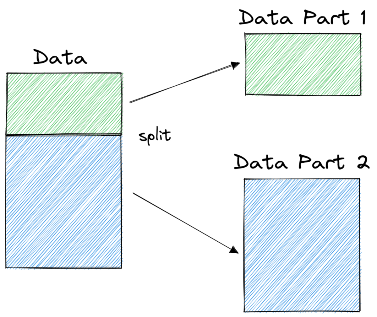
Image by Author
In the picture above, you can see one example of a split — the original dataset gets separated into two parts. In the next step, both of these parts get split again, and so on. This continues until some kind of stopping criterion is met, for example,
- if the split results in a part being empty
- if a certain recursion depth was reached
- if (after previous splits) the dataset only consists of only a few elements, making further splits unnecessary.
How do we find these splits? And why do we even care? Let’s find out.
Motivation
Let us assume that we want to solve a binary classification problem that we create ourselves now:
import numpy as np
np.random.seed(0)

X = np.random.randn(100, 2) # features
y = ((X[:, 0] > 0) * (X[:, 1] < 0)) # labels (0 and 1)
The two-dimensional data looks like this:
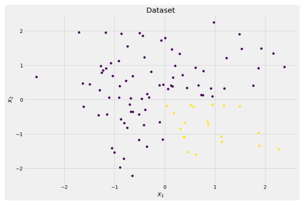
Image by Author
We can see that there are two different classes — purple in about 75% and yellow in about 25% of the cases. If you feed this data to a decision tree classifier, this tree has the following thoughts initially:
“There are two different labels, which is too messy for me. I want to clean up this mess by splitting the data into two parts —these parts should be cleaner than the complete data before.” — tree that gained consciousness
And so the tree does.
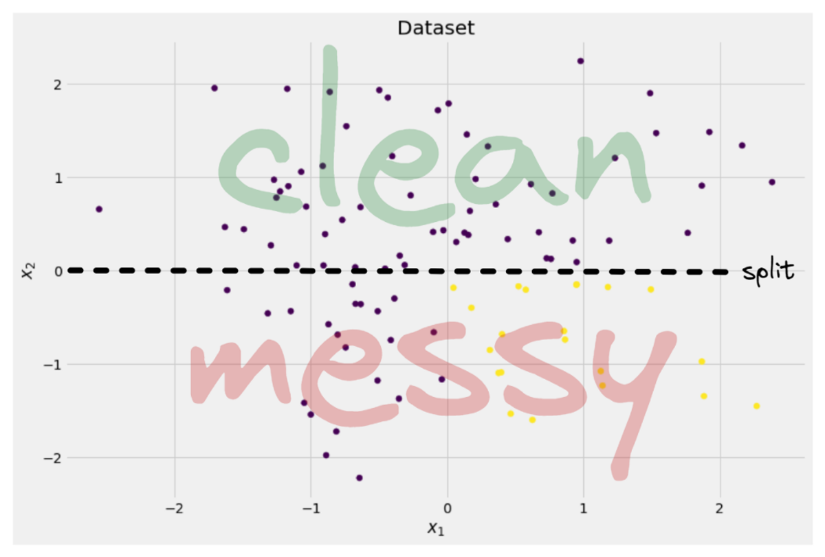
Image by Author
The tree decides to make a split approximately along the x-axis. This has the effect that the top part of the data is now perfectly clean, meaning that you only find a single class (purple in this case) there.
However, the bottom part is still messy, even messier than before in a sense. The class ratio used to be around 75:25 in the complete dataset, but in this smaller part it is about 50:50, which is as mixed up as it can get
Note: Here, it doesn’t matter that the purple and yellow are nicely separated in the picture. Just the raw amout of different labels in the two parts count.
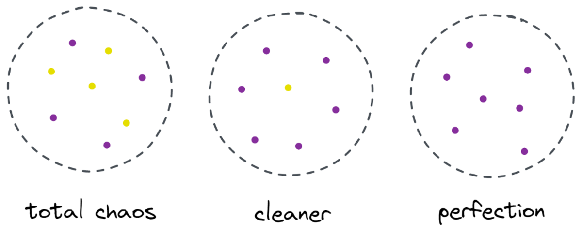
Image by Author
Still, this is good enough as a first step for the tree, and so it carries on. While it wouldn’t create another split in the top, clean part anymore, it can create another split in the bottom part to clean it up.
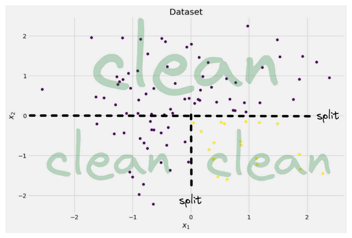
Image by Author
Et voilà, each of the three separate parts is completely clean, as we only find a single color (label) per part.
It is really easy to make predictions now: If a new data point comes in, you just check in which of the three parts it lies and give it the corresponding color. This works so well now because each part is clean. Easy, right?
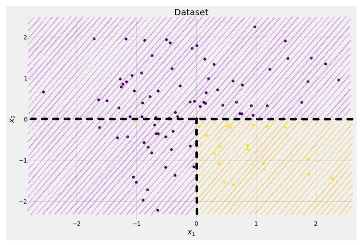
Image by Author
Alright, we were talking about clean and messy data but so far these words only represent some vague idea. In order to implement anything, we have to find a way to define cleanliness.
Measures for Cleanliness
Let us assume that we have some labels, for example
y_1 = [0, 0, 0, 0, 0, 0, 0, 0]

y_2 = [1, 0, 0, 0, 0, 0, 1, 0]
y_3 = [1, 0, 1, 1, 0, 0, 1, 0]
Intuitively, y₁ is the cleanest set of labels, followed by y₂ and then y₃. So far so good, but how can we put numbers on this behavior? Maybe the easiest thing that comes to mind is the following:
Just count the amount of zeroes and amount of ones. Compute their absolute difference. To make it nicer, normalize it by dividing through the length of the arrays.
For example, y₂ has 8 entries in total — 6 zeroes and 2 ones. Hence, our custom-defined cleanliness score would be |6 - 2| / 8 = 0.5. It is easy to calculate that cleanliness scores of y₁ and y₃ are 1.0 and 0.0 respectively. Here, we can see the general formula:
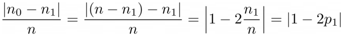
Image by Author
Here, n₀ and n₁ are the numbers of zeroes and ones respectively, n = n₀ + n₁ is the length of the array and p₁ = n₁ / n is the share of the 1 labels.
The problem with this formula is that it is specifically tailored to the case of two classes, but very often we are interested in multi-class classification. One formula that works quite well is the Gini impurity measure:

Image by Author
or the general case:
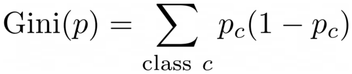
Image by Author
It works so well that scikit-learn adopted it as the default measure for its DecisionTreeClassifier class.
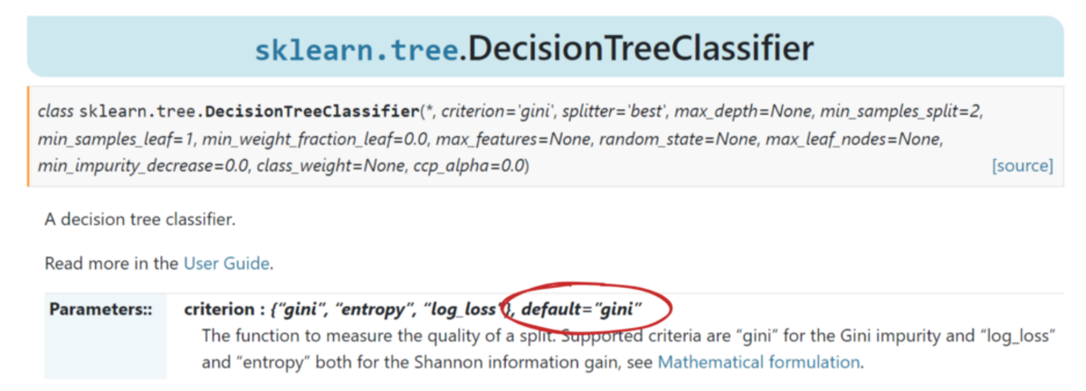
Image by Author
Note: Gini measures messiness instead of cleanliness. Example: if a list only conains a single class (=very clean data!), then all terms in the sum are zero, hence the sum is zero. The worst case is if all classes appear the exact number of times, in which case the Gini is 1–1/C where C is the number of classes.
Now that we have a measure for cleanliness/messiness, let us see how it can be used to find good splits.
Finding Splits
There are a lot of splits we choose from, but which is a good one? Let us use our initial dataset again, together with the Gini impurity measure.

Image by Author
We won’t count the points now, but let us assume that 75% are purple and 25% are yellow. Using the definition of Gini, the impurity of the complete dataset is

Image by Author
If we split the dataset along the x-axis, as done before:
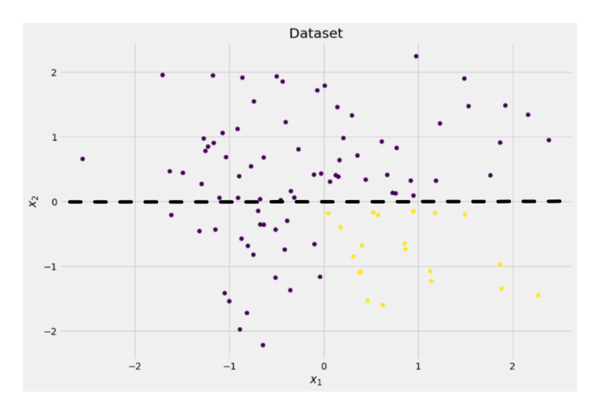
Image by Author
The top part has a Gini impurity of 0.0 and the bottom part

Image by Author
On average, the two parts have a Gini impurity of (0.0 + 0.5) / 2 = 0.25, which is better than the entire dataset’s 0.375 from before. We can also express it in terms of the so-called information gain:
The information gain of this split is 0.375 – 0.25 = 0.125.
Easy as that. The higher the information gain (i.e. the lower the Gini impurity), the better.
Note: Another equally good initial split would be along the y-axis.
An important thing to keep in mind is that it is useful to weigh the Gini impurities of the parts by the size of the parts. For example, let us assume that
- part 1 consists of 50 datapoints and has a Gini impurity of 0.0 and
- part 2 consists of 450 datapoints and has a Gini impurity of 0.5,
then the average Gini impurity should not be (0.0 + 0.5) / 2 = 0.25 but rather 50 / (50 + 450) * 0.0 + 450 / (50 + 450) * 0.5 = 0.45.
Okay, and how do we find the best split? The simple but sobering answer is:
Just try out all the splits and pick the one with the highest information gain. It’s basically a brute-force approach.
To be more precise, standard decision trees use splits along the coordinate axes, i.e. xᵢ = c for some feature i and threshold c. This means that
- one part of the split data consists of all data points x with xᵢ < cand
- the other part of all points x with xᵢ ≥ c.
These simple splitting rules have proven good enough in practice, but you can of course also extend this logic to create other splits (i.e. diagonal lines like xᵢ + 2xⱼ = 3, for example).
Great, these are all the ingredients that we need to get going now!
The Implementation
We will implement the decision tree now. Since it consists of nodes, let us define a Node class first.
from dataclasses import dataclass

@dataclass
class Node:
    feature: int = None # feature for the split
    value: float = None # split threshold OR final prediction
    left: np.array = None # store one part of the data
    right: np.array = None # store the other part of the data
A node knows the feature it uses for splitting (feature) as well as the splitting value (value). value is also used as a storage for the final prediction of the decision tree. Since we will build a binary tree, each node needs to know its left and right children, as stored in left and right .
Now, let’s do the actual decision tree implementation. I’m making it scikit-learn compatible, hence I use some classes from sklearn.base . If you are not familiar with that, check out my article about how to build scikit-learn compatible models.
Let’s implement!
import numpy as np
from sklearn.base import BaseEstimator, ClassifierMixin


class DecisionTreeClassifier(BaseEstimator, ClassifierMixin):
    def __init__(self):
        self.root = Node()

    @staticmethod
    def _gini(y):
        """Gini impurity."""
        counts = np.bincount(y)
        p = counts / counts.sum()

        return (p * (1 - p)).sum()

    def _split(self, X, y):
        """Bruteforce search over all features and splitting points."""
        best_information_gain = float("-inf")
        best_feature = None
        best_split = None

        for feature in range(X.shape[1]):
            split_candidates = np.unique(X[:, feature])
            for split in split_candidates:
                left_mask = X[:, feature] < split
                X_left, y_left = X[left_mask], y[left_mask]
                X_right, y_right = X[~left_mask], y[~left_mask]

                information_gain = self._gini(y) - (
                    len(X_left) / len(X) * self._gini(y_left)
                    + len(X_right) / len(X) * self._gini(y_right)
                )

                if information_gain > best_information_gain:
                    best_information_gain = information_gain
                    best_feature = feature
                    best_split = split

        return best_feature, best_split

    def _build_tree(self, X, y):
        """The heavy lifting."""
        feature, split = self._split(X, y)

        left_mask = X[:, feature] < split

        X_left, y_left = X[left_mask], y[left_mask]
        X_right, y_right = X[~left_mask], y[~left_mask]

        if len(X_left) == 0 or len(X_right) == 0:
            return Node(value=np.argmax(np.bincount(y)))
        else:
            return Node(
                feature,
                split,
                self._build_tree(X_left, y_left),
                self._build_tree(X_right, y_right),
            )

    def _find_path(self, x, node):
        """Given a data point x, walk from the root to the corresponding leaf node. Output its value."""
        if node.feature == None:
            return node.value
        else:
            if x[node.feature] < node.value:
                return self._find_path(x, node.left)
            else:
                return self._find_path(x, node.right)

    def fit(self, X, y):
        self.root = self._build_tree(X, y)
        return self

    def predict(self, X):
        return np.array([self._find_path(x, self.root) for x in X])
And that’s it! You can do all of the things that you love about scikit-learn now:
dt = DecisionTreeClassifier().fit(X, y)
print(dt.score(X, y)) # accuracy

# Output
# 1.0
Since the tree is unregularized, it is overfitting a lot, hence the perfect train score. The accuracy would be worse on unseen data. We can also check how the tree looks like via
print(dt.root)

# Output (prettified manually):
# Node(
#   feature=1,
#   value=-0.14963454032767076,
#   left=Node(
#          feature=0,
#          value=0.04575851730144607,
#          left=Node(
#                 feature=None,
#                 value=0,
#                 left=None,
#                 right=None
#          ),
#          right=Node(
#                  feature=None,
#                  value=1,
#                  left=None,
#                  right=None
#          )
#        ),
#   right=Node(
#           feature=None,
#           value=0,
#           left=None,
#           right=None
#   )
# )
As a picture, it would be this:
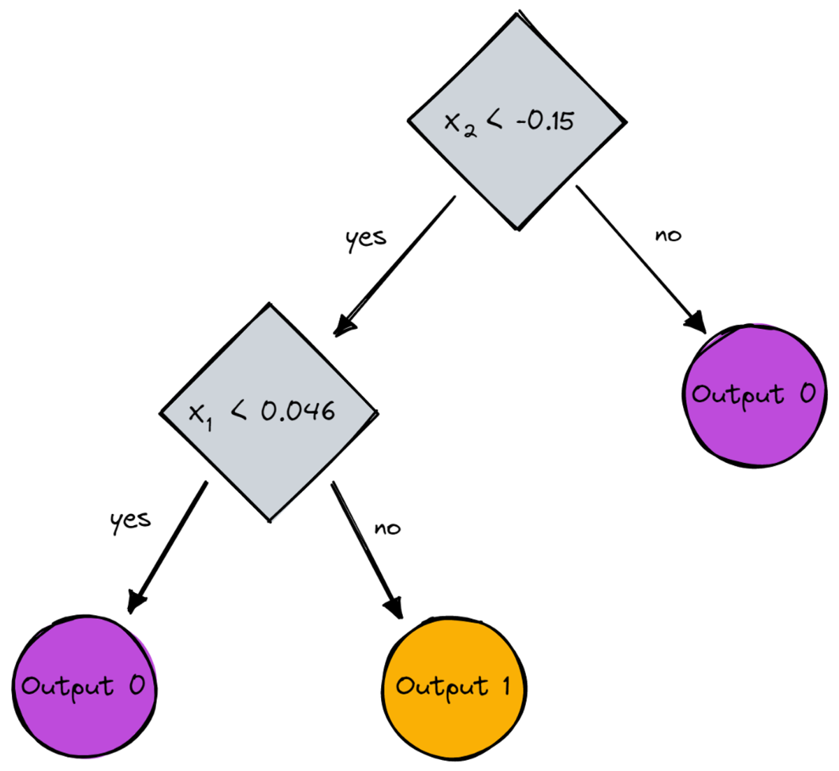
Image by Author
Conclusion
In this article, we have seen how decision trees work in detail. We started out with some vague, yet intuitive ideas and turned them into formulas and algorithms. In the end, we were able to implement a decision tree from scratch.
A word of caution though: Our decision tree cannot be regularized yet. Usually, we would like to specify parameters like
- max depth
- leaf size
- and minimal information gain
among many others. Luckily, these things are not that difficult to implement, which makes this a perfect homework for you. For example, if you specify leaf_size=10 as a parameter, then nodes containing more than 10 samples should not be split anymore. Also, this implementation is not efficient. Usually, you would not want to store parts of the datasets in nodes, but only the indices instead. So your (potentially large) dataset is in memory only once.
The good thing is that you can go crazy now with this decision tree template. You can:
- implement diagonal splits, i.e. xᵢ + 2xⱼ = 3 instead of just xᵢ = 3,
- change the logic that happens inside of the leaves, i.e. you can run a logistic regression within each leaf instead of just doing a majority vote, which gives you a linear tree
- change the splitting procedure, i.e. instead of doing brute force, try some random combinations and pick the best one, which gives you an extra-tree classifier
- and more.
Dr. Robert Kübler is a Senior Data Scientist at METRO.digital and Author at Towards Data Science.
Original. Reposted with permission.