Schedule & Run ETLs with Jupysql and GitHub Actions
This blog provided you with a comprehensive overview of ETL and JupySQL, including a brief introduction to ETLs and JupySQL. We also demonstrated how to schedule an example ETL notebook via GitHub actions, which allows you to automate the process of executing ETLs and JupySQL from Jupyter.
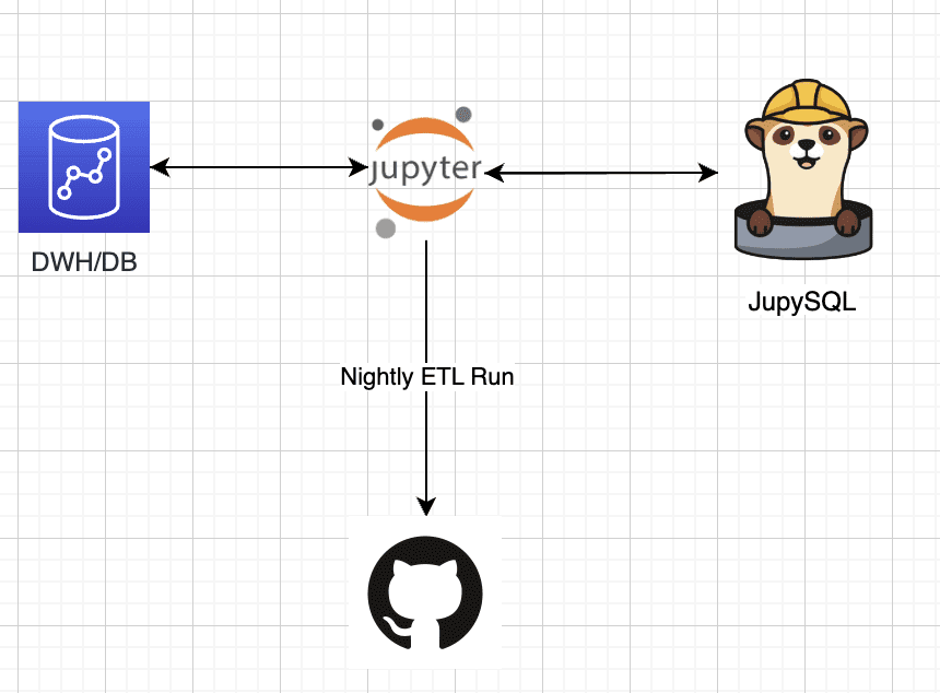
Image by Author
In this blog you'll achieve:
- Have a basic understanding of ETLs and JupySQL
- Use the public Penguins dataset and perform ETL.
- Schedule the ETL we've built on GitHub actions.
Introduction
In this brief yet informative guide, we aim to provide you with a comprehensive understanding of the fundamental concepts of ETL (Extract, Transform, Load) and JupySQL, a flexible and versatile tool that allows for seamless SQL-based ETL from Jupyter.
Our primary focus will be on demonstrating how to effectively execute ETLs through JupySQL, the popular and powerful Python library designed for SQL interaction, while also highlighting the benefits of automating the ETL process through scheduling a full example ETL notebook via GitHub actions.
But first, what is an ETL?
Now, let's dive into the details. ETL (Extract, Transform, Load) crucial process in data management that involves the extraction of data from various sources, the transformation of the extracted data into a usable format, and loading the transformed data into a target database or data warehouse. It is an essential process for data analysis, data science, data integration, and data migration, among other purposes. On the other hand, JupySQL is a widely-used Python library that simplifies the interaction with databases through the power of SQL queries. By using JupySQL, data scientists and analysts can easily execute SQL queries, manipulate data frames, and interact with databases from their Jupyter notebooks.
Why ETLs are important?
ETLs play a significant role in data analytics and business intelligence. They help businesses to collect data from various sources, including social media, web pages, sensors, and other internal and external systems. By doing this, businesses can obtain a holistic view of their operations, customers, and market trends.
After extracting data, ETLs transform it into a structured format, such as a relational database, which allows businesses to analyze and manipulate data easily. By transforming data, ETLs can clean, validate, and standardize it, making it easier to understand and analyze.
Finally, ETLs load the data into a database or data warehouse, where businesses can access it easily. By doing this, ETLs enable businesses to access accurate and up-to-date information, allowing them to make informed decisions.
What is JupySQL?
JupySQL is an extension for Jupyter Notebooks that allows you to interact with databases using SQL queries. It provides a convenient way to access databases and data warehouses directly from Jupyter Notebooks, allowing you to perform complex data manipulations and analyses.
JupySQL supports multiple database management systems, including SQLite, MySQL, PostgreSQL, DuckDB, Oracle, Snowflake and more (check out our integrations section on the left to learn more). You can connect to databases using standard connection strings or through the use of environment variables.
Why JupySQL?
JupySQL, a powerful tool, facilitates direct SQL query interaction with databases inside Jupyter notebooks. With a view to carrying out efficient and accurate data extraction and transformation processes, there are several critical factors to consider when performing ETLs via JupySQL. JupySQL provides users with the necessary tools to interact with data sources and perform data transformations with ease. To save valuable time and effort while guaranteeing consistency and reliability, automating the ETL process through scheduling a full ETL notebook via GitHub actions can be a game-changer. By utilizing JupySQL, users can achieve the best of both worlds, data interactivity (Jupyter) and ease of usage and SQL connectivity (JupySQL), thereby streamlining the data management process and allowing data scientists and analysts to concentrate on their core competencies - generating valuable insights and reports.
Getting started with JupySQL
To use JupySQL, you need to install it using pip. You can run the following command:
!pip install jupysql --quiet
Once installed, you can load the extension in Jupyter notebooks using the following command:
%load_ext sql
After loading the extension, you can connect to a database using the following command:
%sql dialect://username:password@host:port/database
For example, to connect to a local DuckDB database, you can use the following command:
%sql duckdb://
Performing ETL using JupySQL
To perform ETLs using JupySQL, we will follow the standard ETL process, which involves the following steps:
- Extract data
- Transform data
- Load data
- Extract data
Extract data
To extract data using JupySQL, we need to connect to the source database and execute a query to retrieve the data. For example, to extract data from a MySQL database, we can use the following command:
%sql mysql://username:password@host:port/database
data = %sql SELECT * FROM mytable
This command connects to the MySQL database using the specified connection string and retrieves all the data from the "mytable" table. The data is stored in the "data" variable as a Pandas DataFrame.
Note: We can also use %%sql df << to save the data into the df variable
Since we'll be running locally via DuckDB we can simply Extract a public dataset and start working immediately. We're going to get our sample dataset (we will work with the Penguins datasets via a csv file):
from urllib.request import urlretrieve

_ = urlretrieve(
   "https://raw.githubusercontent.com/mwaskom/seaborn-data/master/penguins.csv",
   "penguins.csv",
)
And we can get a sample of the data to check we're connected and we can query the data:
SELECT *
FROM penguins.csv
LIMIT 3
Transform data
After extracting data, it's often necessary to transform it into a format that's more suitable for analysis. This step may include cleaning data, filtering data, aggregating data, and combining data from multiple sources. Here are some common data transformation techniques:
- Cleaning data: Data cleaning involves removing or fixing errors, inconsistencies, or missing values in the data. For example, you might remove rows with missing values, replace missing values with the mean or median value, or fix typos or formatting errors.
- Filtering data: Data filtering involves selecting a subset of data that meets specific criteria. For example, you might filter data to only include records from a specific date range, or records that meet a certain threshold.
- Aggregating data: Data aggregation involves summarizing data by calculating statistics such as the sum, mean, median, or count of a particular variable. For example, you might aggregate sales data by month or by product category.
- Combining data: Data combination involves merging data from multiple sources to create a single dataset. For example, you might combine data from different tables in a relational database, or combine data from different files.
In JupySQL, you can use Pandas DataFrame methods to perform data transformations or native SQL. For example, you can use the rename method to rename columns, the dropna method to remove missing values, and the astype method to convert data types. I'll demonstrate how to do it either with pandas or SQL.
- Note: You can use either
%sqlor%%sql, check out the difference between the two here
Here's an example of how to use Pandas and the JupySQL alternatives to transform data:
# Rename columns
df = data.rename(columns={'old_column_name': 'new_column_name'})  # Pandas
%%sql df <<
SELECT *, old_column_name
AS new_column_name
FROM data;  # JupySQL
# Remove missing values
data = data.dropna()  # Pandas
%%sql df <<
SELECT *
FROM data
WHERE column_name IS NOT NULL;  # JupySQL single column, can add conditions to all columns as needed.
# Convert data types
data['date_column'] = data['date_column'].astype('datetime64[ns]')  # Pandas
%sql df <<
SELECT *,
CAST(date_column AS timestamp) AS date_column
FROM data  # Jupysql
# Filter data
filtered_data = data[data['sales'] > 1000]  # Pandas
%%sql df <<
SELECT * FROM data
WHERE sales > 1000;  # JupySQL
# Aggregate data
monthly_sales = data.groupby(['year', 'month'])['sales'].sum()  # Pandas
%%sql df <<
SELECT year, month,
SUM(sales) as monthly_sales
FROM data
GROUP BY year, month  # JupySQL
# Combine data
merged_data = pd.merge(data1, data2, on='key_column')  # Pandas
%%sql df <<
SELECT * FROM data1
JOIN data2
ON data1.key_column = data2.key_column;  # JupySQL
In our example we'll use simple transformations, in a similar manner to the above code. We'll clean our data from NAs and will split a column (species) into 3 individual columns (named for each species):
# Combine data
merged_data = pd.merge(data1, data2, on='key_column')  # Pandas
%%sql df <<
SELECT * FROM data1
JOIN data2
ON data1.key_column = data2.key_column;  # JupySQL
SELECT *
FROM penguins.csv
WHERE species IS NOT NULL AND island IS NOT NULL AND bill_length_mm IS NOT NULL AND bill_depth_mm IS NOT NULL
AND flipper_length_mm IS NOT NULL AND body_mass_g IS NOT NULL AND sex IS NOT NULL;
# Map the species column into classifiers
transformed_df = transformed_df.DataFrame().dropna()
transformed_df["mapped_species"] = transformed_df.species.map(
   {"Adelie": 0, "Chinstrap": 1, "Gentoo": 2}
)
transformed_df.drop("species", inplace=True, axis=1)


# Checking our transformed data
transformed_df.head()
Load data
After transforming the data, we need to load it into a destination database or data warehouse. We can use ipython-sql to connect to the destination database and execute SQL queries to load the data. For example, to load data into a PostgreSQL database, we can use the following command:
%sql postgresql://username:password@host:port/database
%sql DROP TABLE IF EXISTS mytable;
%sql CREATE TABLE mytable (column1 datatype1, column2 datatype2, ...);
%sql COPY mytable FROM '/path/to/datafile.csv' DELIMITER ',' CSV HEADER;
This command connects to the PostgreSQL database using the specified connection string, drops the "mytable" table if it exists, creates a new table with the specified columns and data types, and loads the data from the CSV file.
Since our use case is using DuckDB locally we can simply save the newly created transformed_df into a csv file, but we can also use the snipped above to save it into our DB or DWH depending on our use case.
Run the following step to save the new data as a CSV file:
transformed_df.to_csv("transformed_data.csv")
We can see a new file called transformed_data.csv was created for us. In the next step we'll see how we can automate this process and consume the final file via GitHub.
Scheduling on GitHub actions
The last step in our process is executing the complete notebook via GitHub actions. To do that we can use ploomber-engine which lets you schedule notebooks, along with other notebook capabilities such as profiling, debugging etc. If needed we can pass external parameters to our notebook and make it a generic template.
- Note: Our notebook file is loading a public dataset and saves it after ETL locally, we can easily change it to consume any dataset, and load it to S3, visualize the data as a dashboard and more.
For our example we can use this sample ci.yml file (this is what sets the github workflow in your repository), and put it in our repository, the final file should be located under .github/workflows/ci.yml.
Content of the ci.yml file:
name: CI

on:
 push:
 pull_request:
 schedule:
   - cron: '0 0 4 * *'

# These permissions are needed to interact with GitHub's OIDC Token endpoint.
permissions:
 id-token: write
 contents: read

jobs:
 report:
   runs-on: ubuntu-latest
   steps:
   - uses: actions/checkout@v3
   - name: Set up Python ${{ matrix.python-version }}
     uses: conda-incubator/setup-miniconda@v2
     with:
       python-version: '3.10'
       miniconda-version: latest
       activate-environment: conda-env
       channels: conda-forge, defaults


   - name: Run notebook
     env:
       PLOOMBER_STATS_ENABLED: false
       PYTHON_VERSION: '3.10'
     shell: bash -l {0}
     run: |
       eval "$(conda shell.bash hook)"

       # pip install -r requirements.txt
       pip install jupysql pandas ploomber-engine --quiet
       ploomber-engine --log-output posthog.ipynb report.ipynb

   - uses: actions/upload-artifact@v3
     if: always()
     with:
       name: Transformed_data
       path: transformed_data.csv
In this example CI, I've also added a scheduled trigger, this job will run nightly at 4 am.
Conclusion
ETLs are an essential process for data analytics and business intelligence. They help businesses to collect, transform, and load data from various sources, making it easier to analyze and make informed decisions. JupySQL is a powerful tool that allows you to interact with databases using SQL queries directly in Jupyter notebooks. Combined with Github actions we can create powerful workflows that can be scheduled and help us get the data to its final stage.
By using JupySQL, you can perform ETLs easily and efficiently, allowing you to extract, transform, and load data in a structured format while Github actions allocate compute and set the environment.
Ido Michael co-founded Ploomber to help data scientists build faster. He'd been working at AWS leading data engineering/science teams. Single handedly he built 100’s of data pipelines during those customer engagements together with his team. Originally from Israel, he came to NY for his MS at Columbia University. He focused on building Ploomber after he constantly found that projects dedicated about 30% of their time just to refactor the dev work (prototype) into a production pipeline.