Customer Segmentation in Python: A Practical Approach
So you want to understand your customer base better? Learn how to leverage RFM analysis and K-Means clustering in Python to perform customer segmentation.
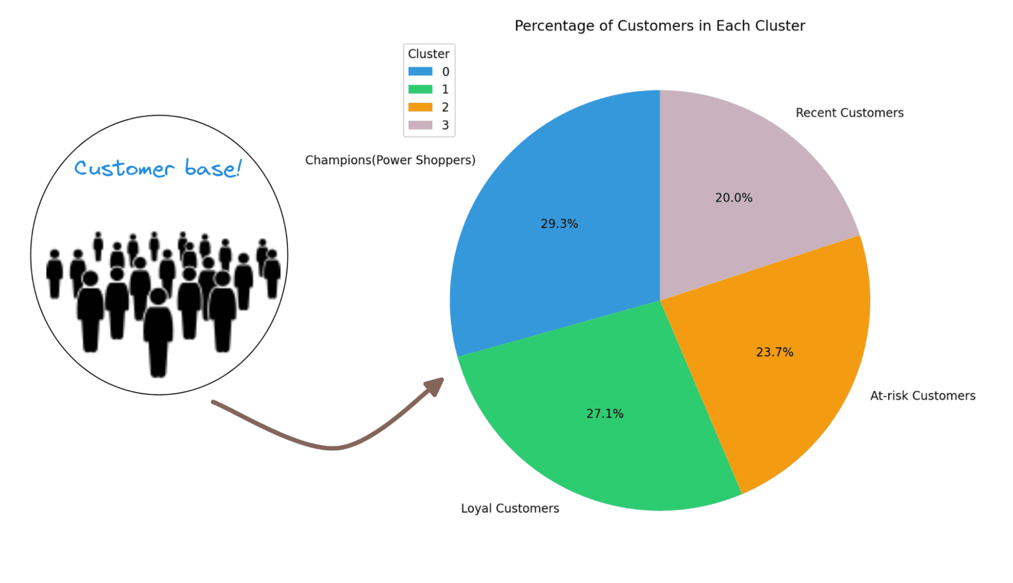
Image by Author | Created Using Excalidraw and Flaticon
Customer segmentation can help businesses tailor their marketing efforts and improve customer satisfaction. Here’s how.
Functionally, customer segmentation involves dividing a customer base into distinct groups or segments—based on shared characteristics and behaviors. By understanding the needs and preferences of each segment, businesses can deliver more personalized and effective marketing campaigns, leading to increased customer retention and revenue.
In this tutorial, we’ll explore customer segmentation in Python by combining two fundamental techniques: RFM (Recency, Frequency, Monetary) analysis and K-Means clustering. RFM analysis provides a structured framework for evaluating customer behavior, while K-means clustering offers a data-driven approach to group customers into meaningful segments. We’ll work with a real-world dataset from the retail industry: the Online Retail dataset from UCI machine learning repository.
From data preprocessing to cluster analysis and visualization, we’ll code our way through each step. So let’s dive in!
Our Approach: RFM Analysis and K-Means Clustering
Let’s start by stating our goal: By applying RFM analysis and K-means clustering to this dataset, we’d like to gain insights into customer behavior and preferences.
RFM Analysis is a simple yet powerful method to quantify customer behavior. It evaluates customers based on three key dimensions:
- Recency (R): How recently did a particular customer make a purchase?
- Frequency (F): How often do they make purchases?
- Monetary Value (M): How much money do they spend?
We’ll use the information in the dataset to compute the recency, frequency, and monetary values. Then, we’ll map these values to the generally used RFM score scale of 1 - 5.
If you’d like, you can explore and analyze further using these RFM scores. But we’ll try to identify customer segments with similar RFM characteristics. And for this, we’ll use K-Means clustering, an unsupervised machine learning algorithm that groups similar data points into clusters.
So let’s start coding!
🔗 Link to Google Colab notebook.
Step 1 – Import Necessary Libraries and Modules
First, let’s import the necessary libraries and the specific modules as needed:
import pandas as pd
import matplotlib.pyplot as plt
from sklearn.cluster import KMeans
We need pandas and matplotlib for data exploration and visualization, and the KMeans class from scikit-learn’s cluster module to perform K-Means clustering.
Step 2 – Load the Dataset
As mentioned, we’ll use the Online Retail dataset. The dataset contains customer records: transactional information, including purchase dates, quantities, prices, and customer IDs.
Let's read in the data that’s originally in an excel file from its URL into a pandas dataframe.
# Load the dataset from UCI repository
url = "https://archive.ics.uci.edu/ml/machine-learning-databases/00352/Online%20Retail.xlsx"
data = pd.read_excel(url)
Alternatively, you can download the dataset and read the excel file into a pandas dataframe.
Step 3 – Explore and Clean the Dataset
Now let’s start exploring the dataset. Look at the first few rows of the dataset:
data.head()
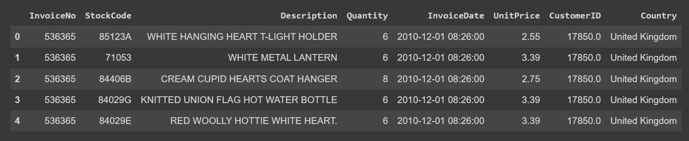
Output of data.head()
Now call the describe() method on the dataframe to understand the numerical features better:
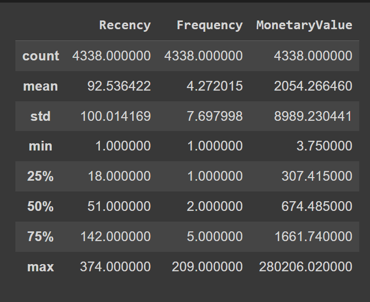
data.describe()
We see that the “CustomerID” column is currently a floating point value. When we clean the data, we’ll cast it into an integer:
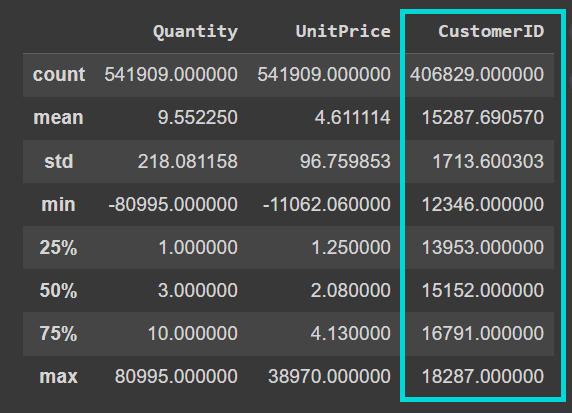
Output of data.describe()
Also note that the dataset is quite noisy. The “Quantity” and “UnitPrice” columns contain negative values:
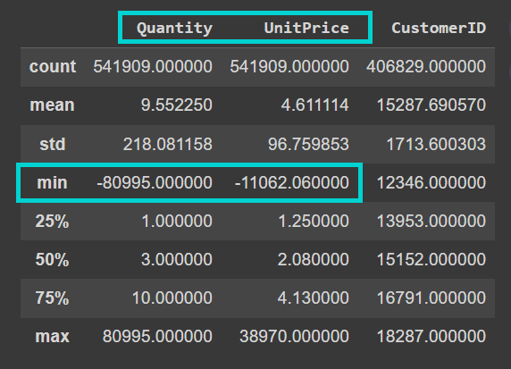
Output of data.describe()
Let’s take a closer look at the columns and their data types:
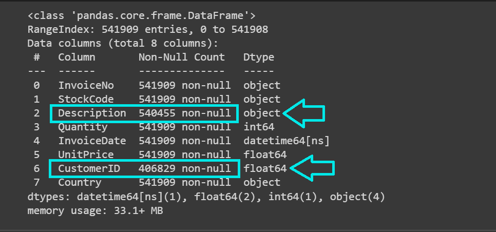
data.info()
We see that the dataset has over 541K records and the “Description” and “CustomerID” columns contain missing values:
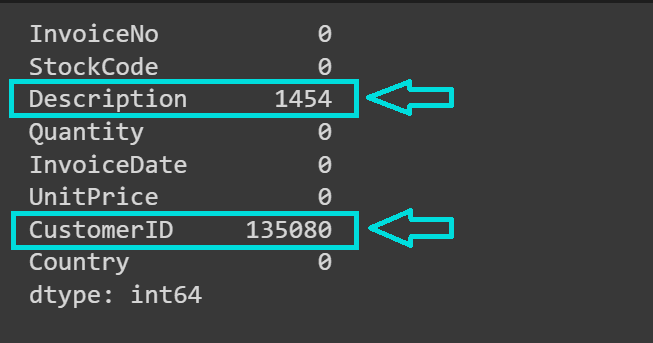
Let’s get the count of missing values in each column:
# Check for missing values in each column
missing_values = data.isnull().sum()
print(missing_values)
As expected, the “CustomerID” and “Description” columns contain missing values:
For our analysis, we don’t need the product description contained in the “Description” column. However, we need the “CustomerID” for the next steps in our analysis. So let’s drop the records with missing “CustomerID”:
# Drop rows with missing CustomerID
data.dropna(subset=['CustomerID'], inplace=True)
Also recall that the values “Quantity” and “UnitPrice” columns should be strictly non-negative. But they contain negative values. So let's also drop the records with negative values for “Quantity” and “UnitPrice”:
# Remove rows with negative Quantity and Price
data = data[(data['Quantity'] > 0) & (data['UnitPrice'] > 0)]
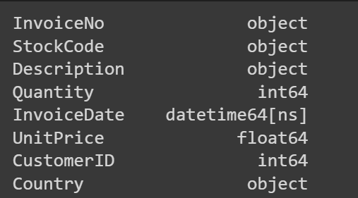
Let’s also convert the “CustomerID” to an integer:
data['CustomerID'] = data['CustomerID'].astype(int)

# Verify the data type conversion
print(data.dtypes)
Step 4 – Compute Recency, Frequency, and Monetary Value
Let’s start out by defining a reference date snapshot_date that’s a day later than the most recent date in the “InvoiceDate” column:
snapshot_date = max(data['InvoiceDate']) + pd.DateOffset(days=1)
Next, create a “Total” column that contains Quantity*UnitPrice for all the records:
data['Total'] = data['Quantity'] * data['UnitPrice']
To calculate the Recency, Frequency, and MonetaryValue, we calculate the following—grouped by CustomerID:
- For recency, we’ll calculate the difference between the most recent purchase date and a reference date (
snapshot_date). This gives the number of days since the customer's last purchase. So smaller values indicate that a customer has made a purchase more recently. But when we talk about recency scores, we’d want customers who bought recently to have a higher recency score, yes? We’ll handle this in the next step. - Because frequency measures how often a customer makes purchases, we’ll calculate it as the total number of unique invoices or transactions made by each customer.
- Monetary value quantifies how much money a customer spends. So we’ll find the average of the total monetary value across transactions.
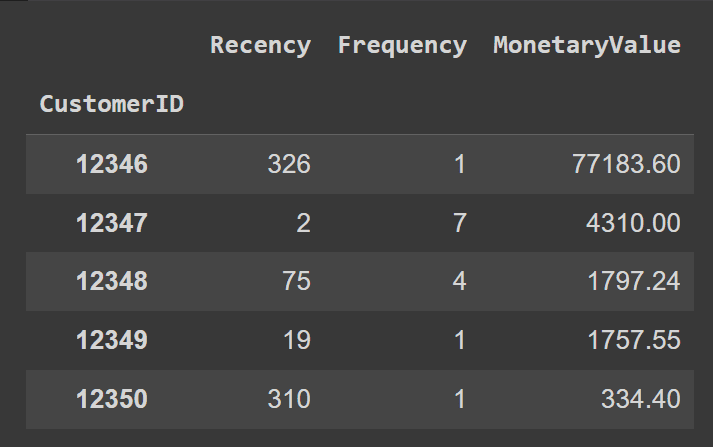
rfm = data.groupby('CustomerID').agg({
    'InvoiceDate': lambda x: (snapshot_date - x.max()).days,
    'InvoiceNo': 'nunique',
    'Total': 'sum'
})
Let’s rename the columns for readability:
rfm.rename(columns={'InvoiceDate': 'Recency', 'InvoiceNo': 'Frequency', 'Total': 'MonetaryValue'}, inplace=True)
rfm.head()
Step 5 – Map RFM Values onto a 1-5 Scale
Now let’s map the “Recency”, “Frequency”, and “MonetaryValue” columns to take on values in a scale of 1-5; one of {1,2,3,4,5}.
We’ll essentially assign the values to five different bins, and map each bin to a value. To help us fix the bin edges, let’s use the quantile values of the “Recency”, “Frequency”, and “MonetaryValue” columns:
rfm.describe()
Here’s how we define the custom bin edges:
# Calculate custom bin edges for Recency, Frequency, and Monetary scores
recency_bins = [rfm['Recency'].min()-1, 20, 50, 150, 250, rfm['Recency'].max()]
frequency_bins = [rfm['Frequency'].min() - 1, 2, 3, 10, 100, rfm['Frequency'].max()]
monetary_bins = [rfm['MonetaryValue'].min() - 3, 300, 600, 2000, 5000, rfm['MonetaryValue'].max()]
Now that we’ve defined the bin edges, let’s map the scores to corresponding labels between 1 and 5 (both inclusive):
# Calculate Recency score based on custom bins
rfm['R_Score'] = pd.cut(rfm['Recency'], bins=recency_bins, labels=range(1, 6), include_lowest=True)

# Reverse the Recency scores so that higher values indicate more recent purchases
rfm['R_Score'] = 5 - rfm['R_Score'].astype(int) + 1

# Calculate Frequency and Monetary scores based on custom bins
rfm['F_Score'] = pd.cut(rfm['Frequency'], bins=frequency_bins, labels=range(1, 6), include_lowest=True).astype(int)
rfm['M_Score'] = pd.cut(rfm['MonetaryValue'], bins=monetary_bins, labels=range(1, 6), include_lowest=True).astype(int)
Notice that the R_Score, based on the bins, is 1 for recent purchases 5 for all purchases made over 250 days ago. But we’d like the most recent purchases to have an R_Score of 5 and purchases made over 250 days ago to have an R_Score of 1.
To achieve the desired mapping, we do: 5 - rfm['R_Score'].astype(int) + 1.
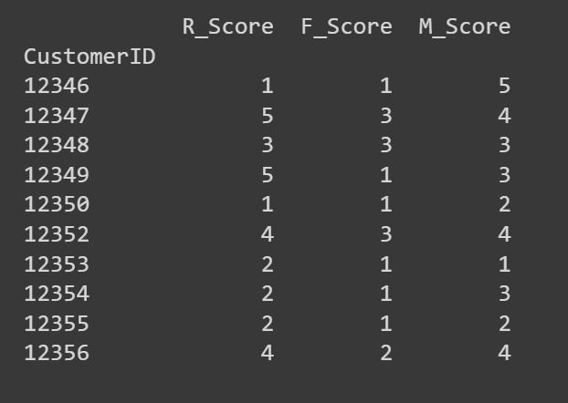
Let’s look at the first few rows of the R_Score, F_Score, and M_Score columns:
# Print the first few rows of the RFM DataFrame to verify the scores
print(rfm[['R_Score', 'F_Score', 'M_Score']].head(10))
If you’d like, you can use these R, F, and M scores to carry out an in-depth analysis. Or use clustering to identify segments with similar RFM characteristics. We’ll choose the latter!
Step 6 – Perform K-Means Clustering
K-Means clustering is sensitive to the scale of features. Because the R, F, and M values are all on the same scale, we can proceed to perform clustering without further scaling the features.
Let’s extract the R, F, and M scores to perform K-Means clustering:
# Extract RFM scores for K-means clustering
X = rfm[['R_Score', 'F_Score', 'M_Score']]
Next, we need to find the optimal number of clusters. For this let’s run the K-Means algorithm for a range of K values and use the elbow method to pick the optimal K:
# Calculate inertia (sum of squared distances) for different values of k
inertia = []
for k in range(2, 11):
kmeans = KMeans(n_clusters=k, n_init= 10, random_state=42)
kmeans.fit(X)
inertia.append(kmeans.inertia_)
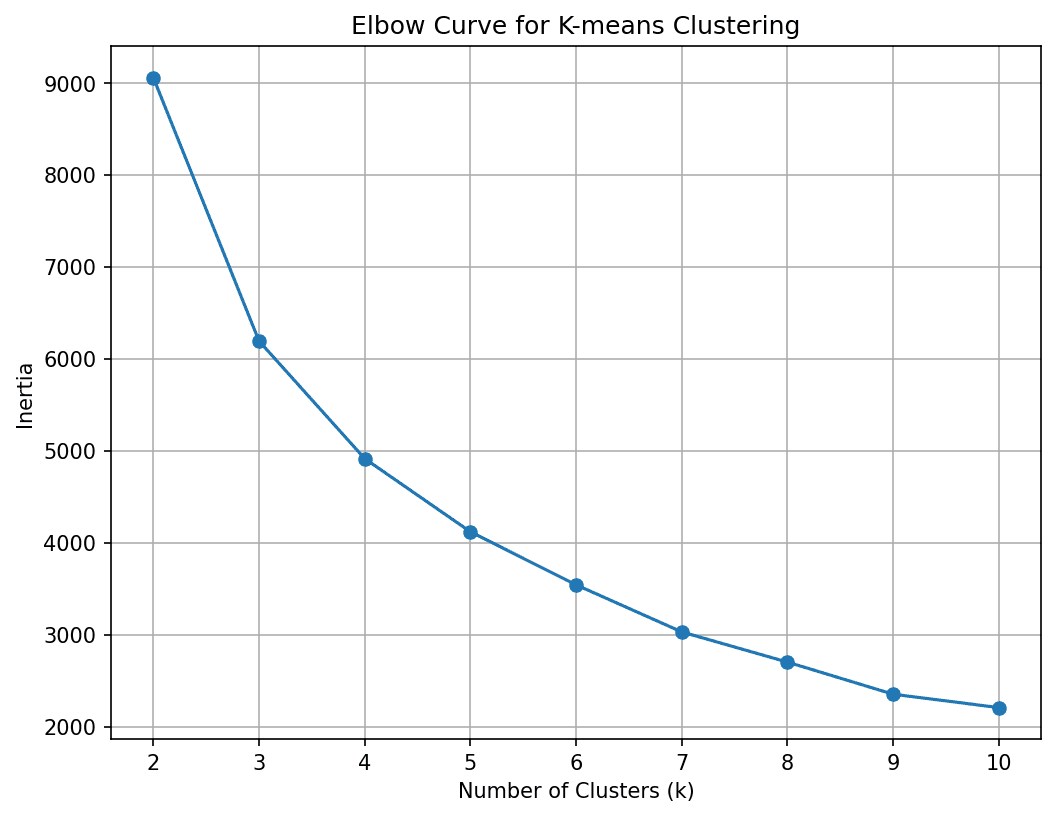
# Plot the elbow curve
plt.figure(figsize=(8, 6),dpi=150)
plt.plot(range(2, 11), inertia, marker='o')
plt.xlabel('Number of Clusters (k)')
plt.ylabel('Inertia')
plt.title('Elbow Curve for K-means Clustering')
plt.grid(True)
plt.show()
We see that the curve elbows out at 4 clusters. So let’s divide the customer base into four segments.
We’ve fixed K to 4. So let’s run the K-Means algorithm to get the cluster assignments for all points in the dataset:
# Perform K-means clustering with best K
best_kmeans = KMeans(n_clusters=4, n_init=10, random_state=42)
rfm['Cluster'] = best_kmeans.fit_predict(X)
Step 7 – Interpret the Clusters to Identify Customer Segments
Now that we have the clusters, let’s try to characterize them based on the RFM scores.
# Group by cluster and calculate mean values
cluster_summary = rfm.groupby('Cluster').agg({
    'R_Score': 'mean',
    'F_Score': 'mean',
    'M_Score': 'mean'
}).reset_index()
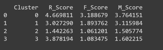
The average R, F, and M scores for each cluster should already give you an idea of the characteristics.
print(cluster_summary)
But let’s visualize the average R, F, and M scores for the clusters so it’s easy to interpret:
colors = ['#3498db', '#2ecc71', '#f39c12','#C9B1BD']

# Plot the average RFM scores for each cluster
plt.figure(figsize=(10, 8),dpi=150)

# Plot Avg Recency
plt.subplot(3, 1, 1)
bars = plt.bar(cluster_summary.index, cluster_summary['R_Score'], color=colors)
plt.xlabel('Cluster')
plt.ylabel('Avg Recency')
plt.title('Average Recency for Each Cluster')

plt.grid(True, linestyle='--', alpha=0.5)
plt.legend(bars, cluster_summary.index, title='Clusters')

# Plot Avg Frequency
plt.subplot(3, 1, 2)
bars = plt.bar(cluster_summary.index, cluster_summary['F_Score'], color=colors)
plt.xlabel('Cluster')
plt.ylabel('Avg Frequency')
plt.title('Average Frequency for Each Cluster')
plt.grid(True, linestyle='--', alpha=0.5)
plt.legend(bars, cluster_summary.index, title='Clusters')

# Plot Avg Monetary
plt.subplot(3, 1, 3)
bars = plt.bar(cluster_summary.index, cluster_summary['M_Score'], color=colors)
plt.xlabel('Cluster')
plt.ylabel('Avg Monetary')
plt.title('Average Monetary Value for Each Cluster')
plt.grid(True, linestyle='--', alpha=0.5)
plt.legend(bars, cluster_summary.index, title='Clusters')

plt.tight_layout()
plt.show()
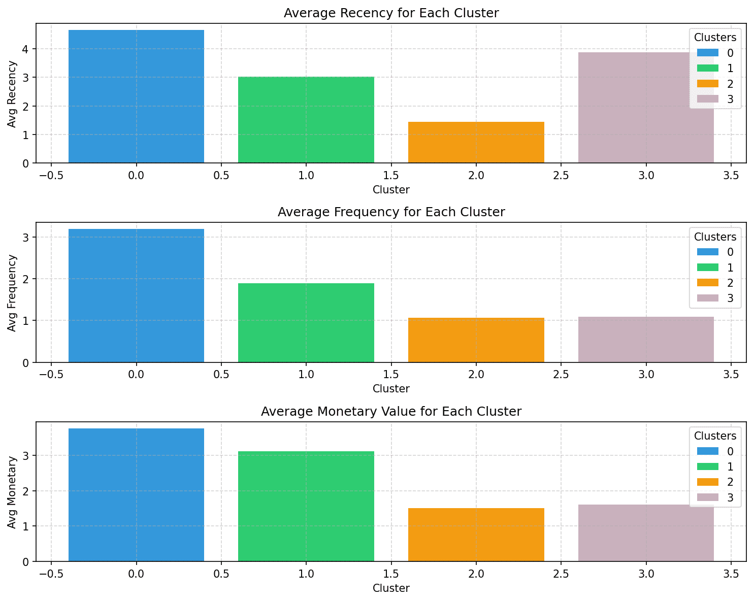
Notice how the customers in each of the segments can be characterized based on the recency, frequency, and monetary values:
- Cluster 0: Of all the four clusters, this cluster has the highest recency, frequency, and monetary values. Let’s call the customers in this cluster champions (or power shoppers).
- Cluster 1: This cluster is characterized by moderate recency, frequency, and monetary values. These customers still spend more and purchase more frequently than clusters 2 and 3. Let’s call them loyal customers.
- Cluster 2: Customers in this cluster tend to spend less. They don’t buy often, and haven’t made a purchase recently either. These are likely inactive or at-risk customers.
- Cluster 3: This cluster is characterized by high recency and relatively lower frequency and moderate monetary values. So these are recent customers who can potentially become long-term customers.
Here are some examples of how you can tailor marketing efforts—to target customers in each segment—to enhance customer engagement and retention:
- For Champions/Power Shoppers: Offer personalized special discounts, early access, and other premium perks to make them feel valued and appreciated.
- For Loyal Customers: Appreciation campaigns, referral bonuses, and rewards for loyalty.
- For At-Risk Customers: Re-engagement efforts that include running discounts or promotions to encourage buying.
- For Recent Customers: Targeted campaigns educating them about the brand and discounts on subsequent purchases.
It’s also helpful to understand what percentage of customers are in the different segments. This will further help streamline marketing efforts and grow your business.
Let’s visualize the distribution of the different clusters using a pie chart:
cluster_counts = rfm['Cluster'].value_counts()

colors = ['#3498db', '#2ecc71', '#f39c12','#C9B1BD']
# Calculate the total number of customers
total_customers = cluster_counts.sum()

# Calculate the percentage of customers in each cluster
percentage_customers = (cluster_counts / total_customers) * 100

labels = ['Champions(Power Shoppers)','Loyal Customers','At-risk Customers','Recent Customers']

# Create a pie chart
plt.figure(figsize=(8, 8),dpi=200)
plt.pie(percentage_customers, labels=labels, autopct='%1.1f%%', startangle=90, colors=colors)
plt.title('Percentage of Customers in Each Cluster')
plt.legend(cluster_summary['Cluster'], title='Cluster', loc='upper left')

plt.show()
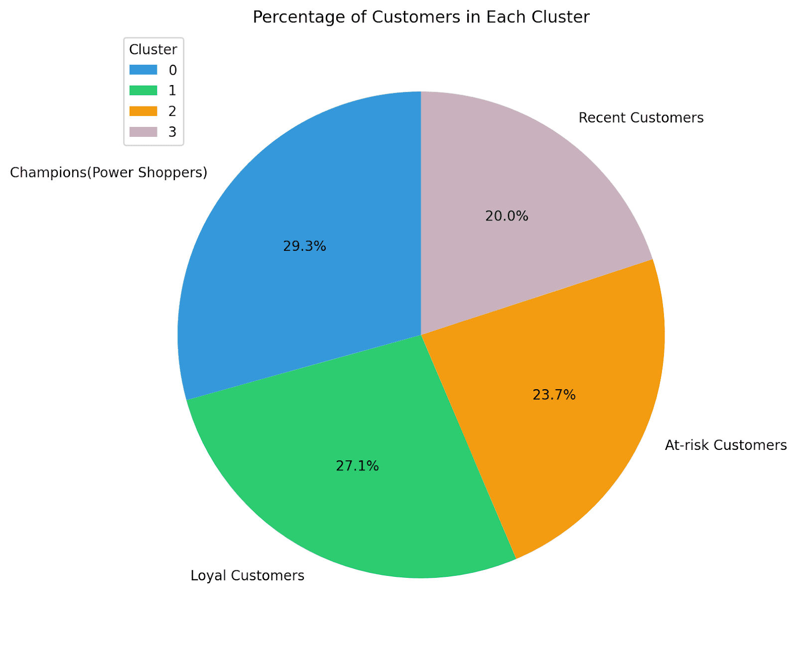
Here we go! For this example, we have quite an even distribution of customers across segments. So we can invest time and effort in retaining existing customers, re-engaging with at-risk customers, and educating recent customers.
Wrapping Up
And that’s a wrap! We went from over 154K customer records to 4 clusters in 7 easy steps. I hope you understand how customer segmentation allows you to make data-driven decisions that influence business growth and customer satisfaction by allowing for:
- Personalization: Segmentation allows businesses to tailor their marketing messages, product recommendations, and promotions to each customer group's specific needs and interests.
- Improved Targeting: By identifying high-value and at-risk customers, businesses can allocate resources more efficiently, focusing efforts where they are most likely to yield results.
- Customer Retention: Segmentation helps businesses create retention strategies by understanding what keeps customers engaged and satisfied.
As a next step, try applying this approach to another dataset, document your journey, and share with the community! But remember, effective customer segmentation and running targeted campaigns requires a good understanding of your customer base—and how the customer base evolves. So it requires periodic analysis to refine your strategies over time.
Dataset Credits
The Online Retail Dataset is licensed under a Creative Commons Attribution 4.0 International (CC BY 4.0) license:
Online Retail. (2015). UCI Machine Learning Repository. https://doi.org/10.24432/C5BW33.
Bala Priya C is a developer and technical writer from India. She likes working at the intersection of math, programming, data science, and content creation. Her areas of interest and expertise include DevOps, data science, and natural language processing. She enjoys reading, writing, coding, and coffee! Currently, she's working on learning and sharing her knowledge with the developer community by authoring tutorials, how-to guides, opinion pieces, and more. Bala also creates engaging resource overviews and coding tutorials.