Mastering Clustering with a Segmentation Problem
The one stop shop for implementing the most widely used models in Python for unsupervised clustering.
By Indraneel Dutta Baruah, AI Driven Solutions Developer

Photo by Mel Poole on Unsplash
In the current age, the availability of granular data for a large pool of customers/products and technological capability to handle petabytes of data efficiently is growing rapidly. Due to this, it’s now possible to come up with very strategic and meaningful clusters for effective targeting. And identifying the target segments requires a robust segmentation exercise. In this blog, we will be discussing the most popular algorithms for unsupervised clustering algorithms and how to implement them in python.
In this blog, we will be working with clickstream data from an online store offering clothing for pregnant women. It includes variables like product category, location of the photo on the webpage, country of origin of the IP address and product price in US dollars. It has data from April 2008 to August 2008.
The first step is to prepare the data for segmentation. I encourage you to check out the article below for an in-depth explanation of different steps for preparing data for segmentation before proceeding further:
One Hot Encoding, Standardization, PCA: Data preparation for segmentation in python
Selecting the optimal number of clusters is another key concept one should be aware of while dealing with a segmentation problem. It will be helpful if you read the article below for understanding a comprehensive list of popular metrics for selecting clusters:
Cheatsheet for implementing 7 methods for selecting the optimal number of clusters in Python
We will be talking about 4 categories of models in this blog:
- K-means
- Agglomerative clustering
- Density-based spatial clustering (DBSCAN)
- Gaussian Mixture Modelling (GMM)
K-means
The K-means algorithm is an iterative process with three critical stages:
1. Pick initial cluster centroids
The algorithm starts by picking initial k cluster centers which are known as centroids. Determining the optimal number of clusters i.e k as well as proper selection of the initial clusters is extremely important for the performance of the model. The number of clusters should always be dependent on the nature of the dataset while poor selection of the initial cluster can lead to the problem of local convergence. Thankfully, we have solutions for both.
For further details on selecting the optimal number of clusters please refer to this detailed blog. For selection of initial clusters, we can either run multiple iterations of the model with various initializations to pick the most stable one or use the “k-means++” algorithm which has the following steps:
- Randomly select the first centroid from the dataset
- Compute distance of all points in the dataset from the selected centroid
- Pick a point as the new centroid that has maximum probability proportional to this distance
- Repeat steps 2 and 3 until k centroids have been sampled
The algorithm initializes the centroids to be distant from each other leading to more stable results than random initialization.
2. Cluster assignment
K-means then assigns the data points to the closest cluster centroids based on euclidean distance between the point and all centroids.
3. Move centroid
The model finally calculates the average of all the points in a cluster and moves the centroid to that average location.
Step 2 and 3 are repeated until there is no change in the clusters or possibly some other stopping condition is met (like maximum number of iterations).
For implementing the model in python we need to do specify the number of clusters first. We have used the elbow method, Gap Statistic, Silhouette score, Calinski Harabasz score and Davies Bouldin score. For each of these methods the optimal number of clusters are as follows:
- Elbow method: 8
- Gap statistic: 29
- Silhouette score: 4
- Calinski Harabasz score: 2
- Davies Bouldin score: 4
As seen above, 2 out of 5 methods suggest that we should use 4 clusters. If each model suggests a different number of clusters we can either take an average or median. The codes for finding the optimal number of k can be found here and further details on each method can be found in this blog.
Once we have the optimal number of clusters, we can fit the model and get the performance of the model using Silhouette score, Calinski Harabasz score and Davies Bouldin score.
# K meansfrom sklearn.cluster import KMeans
from sklearn.metrics import silhouette_score
from sklearn.metrics import calinski_harabasz_score
from sklearn.metrics import davies_bouldin_score# Fit K-Means
kmeans_1 = KMeans(n_clusters=4,random_state= 10)# Use fit_predict to cluster the dataset
predictions = kmeans_1.fit_predict(cluster_df)# Calculate cluster validation metricsscore_kemans_s = silhouette_score(cluster_df, kmeans_1.labels_, metric='euclidean')score_kemans_c = calinski_harabasz_score(cluster_df, kmeans_1.labels_)score_kemans_d = davies_bouldin_score(cluster_df, predictions)print('Silhouette Score: %.4f' % score_kemans_s)
print('Calinski Harabasz Score: %.4f' % score_kemans_c)
print('Davies Bouldin Score: %.4f' % score_kemans_d)
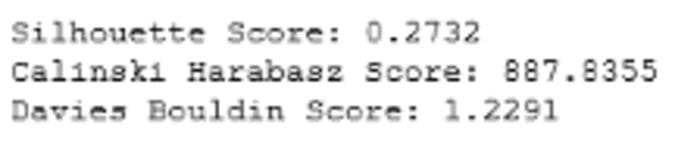
Fig 1: Cluster Validation Metrics for K-Means (Image by author)
We can also check the relative size and distribution of the clusters using an inter-cluster distance map.
# Inter cluster distance map
from yellowbrick.cluster import InterclusterDistance# Instantiate the clustering model and visualizervisualizer = InterclusterDistance(kmeans_1)visualizer.fit(cluster_df)        # Fit the data to the visualizer
visualizer.show()        # Finalize and render the figure
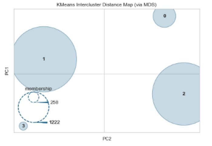
Fig 2: Inter Cluster Distance Map: K-Means (Image by author)
As seen in the figure above, two clusters are quite large compared to the others and they seem to have decent separation between them. However, if two clusters overlap in the 2D space, it does not imply that they overlap in the original feature space. Further details on the model can be found here. Finally, other variants of K-Means like Mini Batch K-means, K-Medoids will be discussed in a separate blog.
Agglomerative clustering
Agglomerative clustering is a general family of clustering algorithms that build nested clusters by merging data points successively. This hierarchy of clusters can be represented as a tree diagram known as dendrogram. The top of the tree is a single cluster with all data points while the bottom contains individual points. There are multiple options for linking data points in a successive manner:
- Single linkage: It minimizes the distance between the closest observations of pairs of clusters
- Complete or Maximum linkage: Tries to minimize the maximum distance between observations of pairs of clusters
- Average linkage: It minimizes the average of the distances between all observations of pairs of clusters
- Ward: Similar to the k-means as it minimizes the sum of squared differences within all clusters but with a hierarchical approach. We will be using this option in our exercise.
The ideal option can be picked by checking which linkage method performs best based on cluster validation metrics (Silhouette score, Calinski Harabasz score and Davies Bouldin score). And similar to K-means, we will have to specify the number of clusters in this model and the dendrogram can help us do that.
# Dendrogram for Hierarchical Clustering
import scipy.cluster.hierarchy as shc
from matplotlib import pyplot
pyplot.figure(figsize=(10, 7))
pyplot.title("Dendrograms")
dend = shc.dendrogram(shc.linkage(cluster_df, method='ward'))
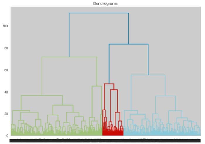
Fig 3: Dendrogram (Image by author)
From figure 3, we can see that we can choose either 4 or 8 clusters. We also use the elbow method, Silhouette score and Calinski Harabasz score to find the optimal number of clusters and get the following results:
- Elbow method: 10
- Davies Bouldin score : 8
- Silhouette score: 3
- Calinski Harabasz score: 2
We will go ahead with 8 as both the Davies Bouldin score and dendrogram suggest so. If the metrics give us different number of cluster we can either go ahead with the one suggested by the dendrogram (as it is based on this specific model) or take average/median of all the metrics. The codes for finding the optimal number of clusters can be found here and further details on each method can be found in this blog.
Similar to k means, we can fit the model with the optimal number of clusters as well as linkage type and test its performance using the three metrics used in K-means.
# Agglomerative clustering
from numpy import unique
from numpy import where
from sklearn.cluster import AgglomerativeClustering
from matplotlib import pyplot# define the model
model = AgglomerativeClustering(n_clusters=4)
# fit model and predict clusters
yhat = model.fit(cluster_df)
yhat_2 = model.fit_predict(cluster_df)
# retrieve unique clusters
clusters = unique(yhat)# Calculate cluster validation metricsscore_AGclustering_s = silhouette_score(cluster_df, yhat.labels_, metric='euclidean')score_AGclustering_c = calinski_harabasz_score(cluster_df, yhat.labels_)score_AGclustering_d = davies_bouldin_score(cluster_df, yhat_2)print('Silhouette Score: %.4f' % score_AGclustering_s)
print('Calinski Harabasz Score: %.4f' % score_AGclustering_c)
print('Davies Bouldin Score: %.4f' % score_AGclustering_d)
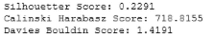
Fig 4: Cluster Validation metrics: Agglomerative Clustering (Image by Author)
Comparing figure 1 and 4, we can see that K-means outperforms agglomerative clustering based on all cluster validation metrics.
Density-based spatial clustering (DBSCAN)
DBSCAN groups together points that are closely packed together while marking others as outliers which lie alone in low-density regions. There are two key parameters in the model needed to define ‘density’: minimum number of points required to form a dense region min_samples and distance to define a neighborhood eps. Higher min_samples or lower eps demands greater density to form a cluster.
Based on these parameters, DBSCAN starts with an arbitrary point x and identifies points that are within neighbourhood of x based on eps and classifies x as one of the following:
- Core point: If the number of points in the neighbourhood is at least equal to the
min_samplesparameter then it called a core point and a cluster is formed around x. - Border point: x is considered a border point if it is part of a cluster with a different core point but number of points in it’s neighbourhood is less than the
min_samplesparameter. Intuitively, these points are on the fringes of a cluster. - Outlier or noise: If x is not a core point and distance from any core sample is at least equal to or greater than
eps, it is considered an outlier or noise.
For tuning the parameters of the model, we first identify the optimal eps value by finding the distance among a point’s neighbors and plotting the minimum distance. This gives us the elbow curve to find density of the data points and optimal eps value can be found at the inflection point. We use the NearestNeighbours function to get the minimum distance and the KneeLocator function to identify the inflection point.
# parameter tuning for eps
from sklearn.neighbors import NearestNeighbors
nearest_neighbors = NearestNeighbors(n_neighbors=11)
neighbors = nearest_neighbors.fit(cluster_df)
distances, indices = neighbors.kneighbors(cluster_df)
distances = np.sort(distances[:,10], axis=0)from kneed import KneeLocator
i = np.arange(len(distances))
knee = KneeLocator(i, distances, S=1, curve='convex', direction='increasing', interp_method='polynomial')
fig = plt.figure(figsize=(5, 5))
knee.plot_knee()
plt.xlabel("Points")
plt.ylabel("Distance")print(distances[knee.knee])
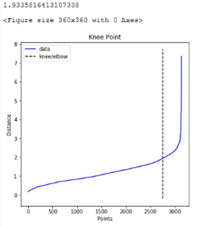
Figure 5: Optimal value for eps (Image by Author)
As seen above, the optimal value for eps is 1.9335816413107338. We use this value for the parameter going forward and try to find the optimal value of min_samples parameter based on Silhouette score, Calinski Harabasz score and Davies Bouldin score. For each of these methods the optimal number of clusters are as follows:
- Silhouette score: 18
- Calinski Harabasz score: 29
- Davies Bouldin score: 2
The codes for finding the optimal number of min_samples can be found here and further details on each method can be found in this blog. We go ahead with the median suggestion which is 18 by Silhouette score.In case we don’t have time to run a grid search over these metrics, one quick rule of thumb is to set min_samples parameter as twice the number of features.
# dbscan clustering
from numpy import unique
from numpy import where
from sklearn.cluster import DBSCAN
from matplotlib import pyplot
# define dataset
# define the model
model = DBSCAN(eps=1.9335816413107338, min_samples= 18)# rule of thumb for min_samples: 2*len(cluster_df.columns)# fit model and predict clusters
yhat = model.fit_predict(cluster_df)
# retrieve unique clusters
clusters = unique(yhat)# Calculate cluster validation metricsscore_dbsacn_s = silhouette_score(cluster_df, yhat, metric='euclidean')score_dbsacn_c = calinski_harabasz_score(cluster_df, yhat)score_dbsacn_d = davies_bouldin_score(cluster_df, yhat)print('Silhouette Score: %.4f' % score_dbsacn_s)
print('Calinski Harabasz Score: %.4f' % score_dbsacn_c)
print('Davies Bouldin Score: %.4f' % score_dbsacn_d)
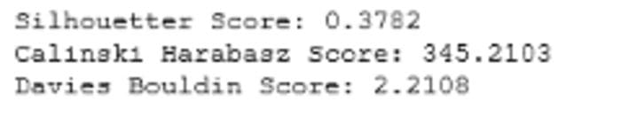
Figure 6: Cluster Validation metrics: DBSCAN (Image by Author)
Comparing figure 1 and 6, we can see that DBSCAN performs better than K-means on Silhouette score. The model is described in the paper:
A Density-Based Algorithm for Discovering Clusters in Large Spatial Databases with Noise, 1996.
In a separate blog, we will be discussing a more advanced version of DBSCAN called Hierarchical Density-Based Spatial Clustering (HDBSCAN).
Gaussian Mixture Modelling (GMM)
A Gaussian mixture model is a distance based probabilistic model that assumes all the data points are generated from a linear combination of multivariate Gaussian distributions with unknown parameters. Like K-means it takes into account centers of the latent Gaussian distributions but unlike K-means, the covariance structure of the distributions is also taken into account. The algorithm implements the expectation-maximization (EM) algorithm to iteratively find the distribution parameters that maximize a model quality measure called log likelihood. The key steps performed in this model are:
- Initialize k gaussian distributions
- Calculate probabilities of each point’s association with each of the distributions
- Recalculate distribution parameters based on each point’s probabilities associated with the the distributions
- Repeat process till log-likelihood is maximized
There are 4 options for calculating covariances in GMM:
- Full: Each distribution has its own general covariance matrix
- Tied: All distributions share general covariance matrix
- Diag: Each distribution has its own diagonal covariance matrix
- Spherical: Each distribution has its own single variance
Apart from selecting the covariance type, we need to select the optimal number of clusters in the model as well. We use BIC score, Silhouette score, Calinski Harabasz score and Davies Bouldin score for selecting both parameters using grid search. For each of these methods the optimal number of clusters are as follows:
- BIC Score: Covariance- ‘full’ and cluster number- 26
- Silhouette score: Covariance- ‘tied’ and cluster number- 2
- Calinski Harabasz score: Covariance- ‘spherical’ and cluster number- 4
- Davies Bouldin score: Covariance- ‘full’ and cluster number- 8
The codes for finding the optimal parameter values can be found here and further details on each method can be found in this blog. We chose covariance as “full” and the number of clusters as 26 based on the BIC score as it is based on this specific model. If we have similar configurations from multiple metrics, we can take average/median/mode of all the metrics. We can now fit the model and check model performance.
# gaussian mixture clustering
from numpy import unique
from numpy import where
from sklearn.mixture import GaussianMixture
from matplotlib import pyplot
# define the model
model = GaussianMixture(n_components= 26,covariance_type= "full", random_state = 10)
# fit the model
model.fit(cluster_df)
# assign a cluster to each example
yhat = model.predict(cluster_df)
# retrieve unique clusters
clusters = unique(yhat)# Calculate cluster validation scorescore_dbsacn_s = silhouette_score(cluster_df, yhat, metric='euclidean')score_dbsacn_c = calinski_harabasz_score(cluster_df, yhat)score_dbsacn_d = davies_bouldin_score(cluster_df, yhat)print('Silhouette Score: %.4f' % score_dbsacn_s)
print('Calinski Harabasz Score: %.4f' % score_dbsacn_c)
print('Davies Bouldin Score: %.4f' % score_dbsacn_d)
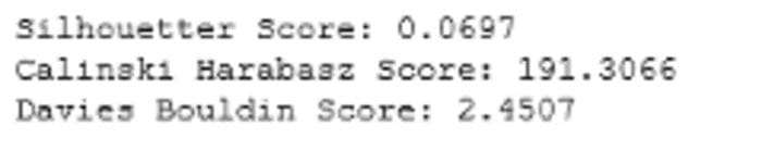
Figure 7: Cluster Validation metrics: GMM (Image by Author)
Comparing figure 1 and 7, we can see that K-means outperforms GMM based on all cluster validation metrics. In a separate blog, we will be discussing a more advanced version of GMM called Variational Bayesian Gaussian Mixture.
Conclusion
The aim of this blog is to help the readers understand how 4 popular clustering models work as well as their detailed implementation in python. As shown below, each model has its own pros and cons:

Fig 8: Pros and Cons of clustering algorithms (Image by Author)
Finally, it is important to understand that these models are just a means to find logical and easily understandable customer/product segments which can be targeted effectively. So in most practical cases, we will end up trying multiple models and creating customer/product profiles from each iteration till we find segments that make the most business sense.Thus, segmentation is both an art and science.
Do you have any questions or suggestions about this blog? Please feel free to drop in a note.
Thank you for reading!
If you, like me, are passionate about AI, Data Science, or Economics, please feel free to add/follow me on LinkedIn, Github and Medium.
References
- Ester, M, Kriegel, H P, Sander, J, and Xiaowei, Xu. A density-based algorithm for discovering clusters in large spatial databases with noise. United States: N. p., 1996. Web.
- MacQueen, J. Some methods for classification and analysis of multivariate observations. Proceedings of the Fifth Berkeley Symposium on Mathematical Statistics and Probability, Volume 1: Statistics, 281–297, University of California Press, Berkeley, Calif., 1967. https://projecteuclid.org/euclid.bsmsp/1200512992
- Scikit-learn: Machine Learning in Python, Pedregosa et al., JMLR 12, pp. 2825–2830, 2011.
Bio: Indraneel Dutta Baruah is striving for excellence in solving business problems using AI!
Original. Reposted with permission.
Related:
- Centroid Initialization Methods for k-means Clustering
- Key Data Science Algorithms Explained: From k-means to k-medoids clustering
- Customer Segmentation Using K Means Clustering