Image by Author

In the present century, data is the new oil. Optimizing this data storage is always critical for getting a good performance from it. Opting for suitable data types and applying the correct normalization process is essential in deciding its performance. 

This article will study the most important and commonly used datatypes and understand the normalization process.

Data Types in SQL

There are mainly two data types in SQL: String and Numeric. Other than this, there are additional data types like Boolean, Date and Time, Array, Interval, XML, etc.

String Data Types

These data types are used to store character strings. The string is often implemented as an array data type and contains a sequence of elements, typically characters.

1. CHAR(n): 

It is a fixed-length string that can contain characters, numbers, and special characters. n denotes the maximum length of the string in characters it can hold.

Its maximum range is from 0 to 255 characters, and the problem with this data type is that it takes the full space specified, even if the actual length of the string is less than then. The extra string length is padded with extra memory space.

2. VARCHAR(n):

Varchar is similar to Char but can support strings of variable size, and there is no padding. The storage size of this data type is equal to the actual length of the string. 

It can store up to a maximum of 65535 characters. Due to its variable size nature, its performance is not as good as the CHAR data type.

3. BINARY(n): 

It is similar to the CHAR data type but only accepts binary strings or binary data. It can be used to store images, files, or any serialized objects. There is another data type VARBINARY(n) which is similar to the VARCHAR data type but also accepts only binary strings or binary data.

4. TEXT(n):

This data type is also used to store the strings but has a maximum size of 65535 bytes.

5. BLOB(n): Stands for Binary Large Object and hold data up to 65535 bytes.

Other than these are other data types, like LONGTEXT and LONGBLOB, which can store even more characters.

Numeric Data Types

1. INT():

It can store a numeric integer, which is 4 bytes (32bit). Here n denotes the display width, which can be a maximum of up to 255. It specifies the minimum number of characters used to display the integer values.

Range:

1. a)  -2147483648 <= Signed INT <= 2147483647
2. b)  0 <= Unsigned INT <= 4294967295

2. BIGINT():

It can store a large integer of size up to 64 bits.

Range:

1. a)  -9223372036854775808 <= Signed BIGINT <= 9223372036854775807
2. b)  0 <= Unsigned BIGINT <= 18446744073709551615

3. FLOAT():

It can store floating point numbers with decimal places approximated with a certain precision. It has some small rounding errors, so because of this, it is not suitable where exact precision is required.

4. DOUBLE():

This data type represents double-precision floating-point numbers. It can store decimal values with a higher precision as compared to the FLOAT data type.

5. DECIMAL(n, d):

This data type represents exact decimal numbers with a fixed precision denoted by d. The parameter d specifies the number of digits after the decimal point, and the parameter n denotes the size of the number. The maximum value for d is 30, and its default value is 0.

Some other Data Types

1. BOOLEAN:

This data type stores only two states which are True or False. It is used to perform logical operations.

2. ENUM:

It stands for Enumeration. It allows you to choose one value from the list of predefined options. It also ensures that the stored value is only from the specified options.

For example, consider an attribute color that can only be 'Red,' 'Green,' or 'Blue'. When we put these values in ENUM, then the value of the color can only be from these specified colors only.

3. XML:

XML stands for eXtensible Markup Language. This data type is used to store XML data which is used for structured data representation.

4. AutoNumber:

It is an integer that automatically increments its value when each record is added. It is used in generating unique or sequential numbers. 

5. Hyperlink:

It can store the hyperlinks of files and web pages.

This completes our discussion on SQL Data Types. There are many more data types, but the data types that we have discussed are the most commonly used ones.

Normalization In SQL

Normalization is the process of removing redundancies, inconsistencies, and anomalies from the database. Redundancy means the presence of duplicate values of the same piece of data, whereas inconsistencies in the database represent the same data exists in multiple formats in multiple tables.

Database anomalies can be defined as any sudden change or discrepancies in the database that are not supposed to exist. These changes can be due to various reasons, such as data corruption, hardware failure, software bugs, etc. Anomalies can lead to severe consequences, such as data loss or inconsistency, so detecting and fixing them as soon as possible is essential. There are mainly three types of anomalies. We will briefly discuss each but refer to this article if you want to read more.

1. Insertion Anomaly:

When the newly inserted row creates, inconsistency in the table leads to an insertion anomaly. For example, we want to add an employee to an organization, but his department is not allocated to him. Then we cannot add that employee to the table, which creates an insertion anomaly.

2. Deletion Anomaly:

Deletion anomaly occurs when we want to delete some rows from the table, and some other data is required to be deleted from the database.

3. Update Anomaly:

This anomaly occurs when we want to update some rows and which leads to inconsistency in the database.

The normalization process contains a series of guidelines that make the design of the database efficient, optimized, and free from redundancies and anomalies. There are several types of normal forms like 1NF, 2NF, 3NF, BCNF, etc.

1. First Normal Form (1NF)

The first normal form ensures that the table contains no composite or multi-valued attributes. It means that only one value is present in a single attribute. A relation is in first normal form if every attribute is only single-valued.

For Ex-

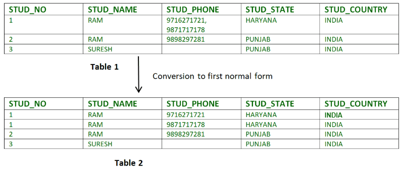
Image by GeeksForGeeks

In Table 1, the attribute STUD_PHONE contains more than one phone number. But in Table 2, this attribute is decomposed into 1st normal form.

2. Second Normal Form

The table must be in the first normal form, and there must not be any partial dependencies in the relations. Partial dependency means that the non-prime attribute (attributes which are not part of the candidate key) is partially dependent or depends on any proper subset of the candidate key. For the relations to be in the second normal form, the non-prime attributes must be fully functional and dependent on the entire candidate key.

For example, consider a table named Employees having the following attributes.

EmployeeID (Primary Key)
ProjectID (Primary Key)
EmployeeName
ProjectName
HoursWorked

Here the EmployeeID and the ProjectID together form the primary key. However, you can notice a partial dependency between EmployeeName and EmployeeID. It means that the EmployeeName is dependent only on the part of the primary key (i.e., EmployeeID). For complete dependency, the EmployeeName must depend on both EmployeeID and the ProjectID. So, this violates the principle of the second normal form.

To make this relation in the second normal form, we must split the tables into two separate tables. The first table contains all the employee details, and the second contains all the project details.

Therefore, the Employee table has the following attributes,

EmployeeID (Primary Key)
EmployeeName

And the Project table has the following attributes,

Project ID (Primary Key)
Project Name
Hours Worked

Now you can see that the partial dependency is removed by creating two independent tables. And the non-prime attributes of both tables depend on the complete set of the primary key.

3. Third Normal Form

After 2NF, still, the relations can have update anomalies. It may happen if we update only one tuple and not the other. That would lead to inconsistency in the database.

The condition for the third normal form is that the table should be in the 2NF, and there is no transitive dependency for the non-prime attributes. Transitive dependency happens when a non-prime attribute depends on another non-prime attribute instead of directly depending on the primary attribute. Prime attributes are the attributes that are part of the candidate key.

Consider a relation R(A, B, C), where A is the primary key and B & C are the non-prime attributes. Let A→B and B→C be two Functional Dependencies, then A→C will be the transitive dependency. It means that attribute C is not directly determined by A. B acts as a middleman between them.

If a table consists of a transitive dependency, then we can bring the table into 3NF by splitting the table into separate independent relations.

4. Boyce-Codd Normal Form

Although 2NF and 3NF remove most of the redundancies, still the redundancies are not 100% removed. Redundancy can occur if the LHS of the functional dependency is not a candidate or super key. A Candidate Key forms from the prime attributes, and the Super Key is a superset of the candidate key. To overcome this issue, another type of functional dependency is available named Boyce Codd Normal Form (BCNF).

For a table to be in BCNF, the left-hand side of a functional dependency must be a candidate key or a super key. A. For example, for a functional dependency X→Y, X must be a candidate or super key.

Consider an Employee Table that contains the following attributes. 

1. Employee ID (primary key)
2. Employee Name
3. Department
4. Department Head

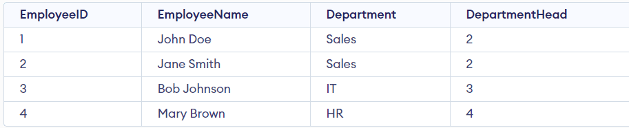
The EmployeeID is the primary key that uniquely identifies each row. The Department attribute represents the department of a particular employee, and the Department Head attribute represents the Employee ID of the employee who is the head of that specific department.

Now we will check if this table is in the BCNF. The condition is that the LHS of the functional dependency must be a super key. Below are the two functional dependencies of that table.

Functional Dependency 1: Employee ID → Employee Name, Department, Department Head

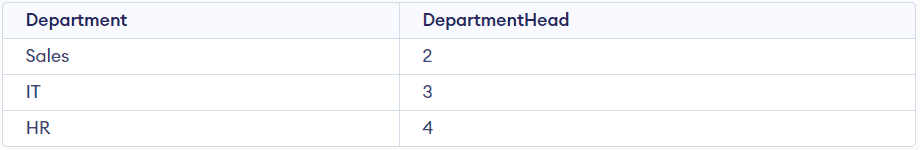
Functional Dependency 2: Department → Department Head

For the FD1, the EmployeeID is the primary key, which is also a super key. But for FD2, Department is not the super key because multiple employees can be in the same department.

Therefore this table violates the condition of BCNF. To satisfy the property of BCNF, we need to split that table into two separate tables: Employees and Departments. The Employees table contains the EmployeeID, EmployeeName, and Department, and the Department table will have the Department and the Department Head.

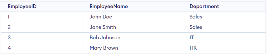
Now we can see in both tables that all the functional dependencies are dependent on the primary keys, i.e., there are no non-trivial dependencies.

We have covered all the famous normalization techniques, but other than these, there are two more normal forms, namely 4NF and 5NF. If you want to read more about them, refer to this article from GeeksForGeeks.

Wrapping it Up

We have discussed the most commonly used data types in SQL and the significant Normalization techniques in database management systems. While designing a database system, we aim to make it scalable, minimizing redundancy and ensuring data integrity.

We can create a delicate balance between storage, precision, and memory consumption by selecting appropriate data types. Also, the normalization process helps eliminate data anomalies and make the schema more organized.

It is all for today. Until then, keep reading and keep learning.
 
 
Aryan Garg is a B.Tech. Electrical Engineering student, currently in the final year of his undergrad. His interest lies in the field of Web Development and Machine Learning. He have pursued this interest and am eager to work more in these directions.