Support Vector Machines: A Concise Technical Overview
Support Vector Machines remain a popular and time-tested classification algorithm. This post provides a high-level concise technical overview of their functionality.
Classification is concerned with building a model that separates data into distinct classes. This model is built by inputting a set of training data for which the classes are pre-labeled in order for the algorithm to learn from. The model is then used by inputting a different dataset for which the classes are withheld, allowing the model to predict their class membership based on what it has learned from the training set. Well-known classification schemes include decision trees and Support Vector Machines, among a whole host of others. As this type of algorithm requires explicit class labeling, classification is a form of supervised learning.
As mentioned, Support Vector Machines (SVMs) are a particular classification strategy. SMVs work by transforming the training dataset into a higher dimension, which is then inspected for the optimal separation boundary, or boundaries, between classes. In SVMs, these boundaries are referred to as hyperplanes, which are identified by locating support vectors, or the instances that most essentially define classes, and their margins, which are the lines parallel to the hyperplane defined by the shortest distance between a hyperplane and its support vectors. Consequently, SVMs are able to classify both linear and nonlinear data.
The grand idea with SVMs is that, with a high enough number of dimensions, a hyperplane separating a particular class from all others can always be found, thereby delineating dataset member classes. When repeated a sufficient number of times, enough hyperplanes can be generated to separate all classes in n-dimensional space. Importantly, SVMs look not just for any separating hyperplane but the maximum-margin hyperplane, being that which resides equidistance from respective class support vectors.
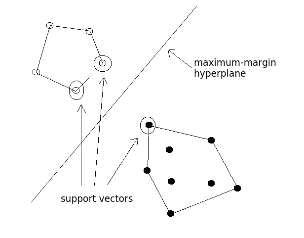
Fig.1: Maximum-Margin Hyperplane and the Support Vectors.
When data is linearly-separable, there are many separating lines that could be chosen. Such a hyperplane can be expressed as

where W is a vector of weights, b is a scalar bias, and X are the training data (of the form (x1, x2 )). If our bias, b, is thought of as an additional weight, the equation can be expressed as

which can, in turn, be rewritten as a pair of linear inequalities, solving to greater or less than zero, either of which satisfied indicate that a particular point lies above or below the hyperplane, respectively. Finding the maximum-margin hyperplane, or the hyperplane that resides equidistance from the support vectors, is done by combining the linear inequalities into a single equation and transforming them into a constrained quadratic optimization problem, using a Lagrangian formulation and solving using Karush-Kuhn-Tucker conditions.
Following this transformation, the maximum-margin hyperplane can be expressed in the form
where b and αi are learned parameters, n is the number of support vectors, i is a support vector instance, t is the vector of training instances, yi is the class value of a particular training instance of vector t, and a(i) is the vector of support vectors. Once the maximum-margin hyperplane is identified and training is complete, only the support vectors are relevant to the model as they define the maximum-margin hyperplane; all of the other training instances can be ignored.
When data is not linearly-separable, the data is first transformed into a higher dimensional space using some function, and this space is then searched for the hyperplane, another quadratic optimization problem. In order to circumvent the additional computational complexity that increased dimensionality brings, all calculations can be performed on the original input data, which is quite likely of lower dimensionality. This higher computational complexity is based on the fact that, in higher dimensionality, the dot product of an instance and each of the support vectors would need to be calculated for each instance classification. A kernel function, which maps an instance to feature space created by a particular function it applies instances to, is used on the original, lower-dimensionality data. A common kernel function is the polynomial kernel, which expressed

computes the dot product of 2 vectors, and raises that result to the power of n.
SVMs are powerful, well-used classification algorithms, which garnered a substantial amount of research attention prior to the deep learning boom we are currently in. Despite the fact that, to the onlooker, they may no longer be bleeding edge algorithms, they certainly have had great success in particular domains, and remain some of the most popular classification algorithms in the toolkits of machine learning practitioners and data scientists.
What has been presented above is a very high-level overview of SVMs. Support Vector Machines are a complex classifier, more of which can be found by starting here.
Related: