 Keep it simple! How to understand Gradient Descent algorithm
 Keep it simple! How to understand Gradient Descent algorithm
In Data Science, Gradient Descent is one of the important and difficult concepts. Here we explain this concept with an example, in a very simple way. Check this out.
By Jahnavi Mahanta.
Source: dilbert.com
When I first started out learning about machine learning algorithms, it turned out to be quite a task to gain an intuition of what the algorithms are doing. Not just because it was difficult to understand all the mathematical theory and notations, but it was also plain boring. When I turned to online tutorials for answers, I could again only see equations or high level explanations without going through the detail in a majority of the cases.
It was then that one of my data science colleagues introduced me to the concept of working out an algorithm in an excel sheet. And that worked wonders for me. Any new algorithm, I try to learn it in an excel at a small scale and believe me, it does wonders to enhance your understanding and helps you fully appreciate the beauty of the algorithm.
Let me explain to you using an example.
Most of the data science algorithms are optimization problems and one of the most used algorithms to do the same is the Gradient Descent Algorithm.
Now, for a starter, the name itself Gradient Descent Algorithm may sound intimidating, well, hopefully after going though this post,that might change.
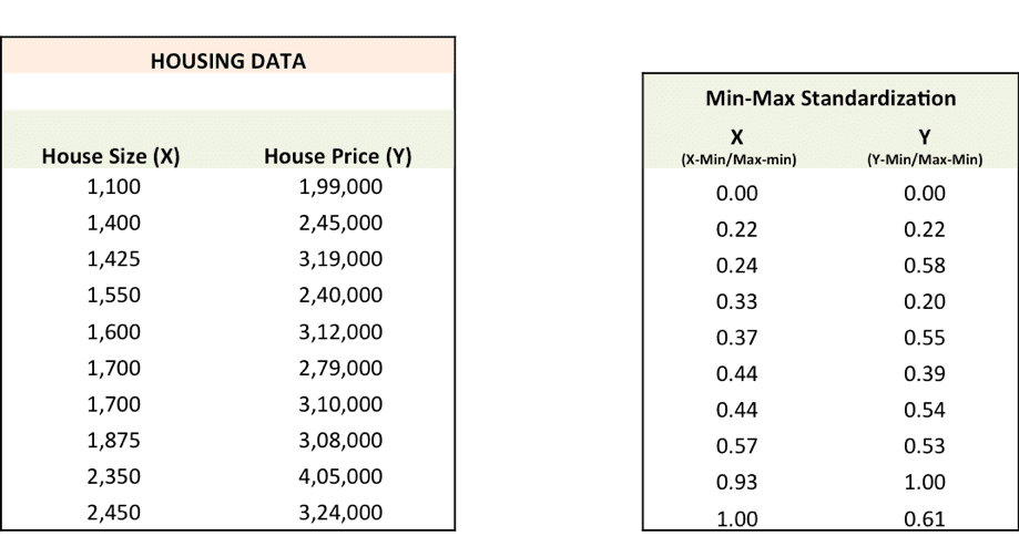
Lets take the example of predicting the price of a new price from housing data:
Now, given historical housing data,the task is to create a model that predicts the price of a new house given the house size.
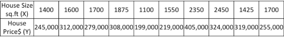
The task – for a new house, given its size (X), what will its price (Y) be?
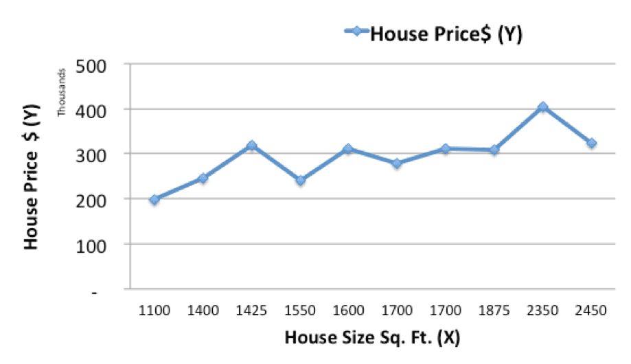
Lets start off by plotting the historical housing data:
Now, we will use a simple linear model, where we fit a line on the historical data, to predict the price of a new house (Ypred) given its size (X)
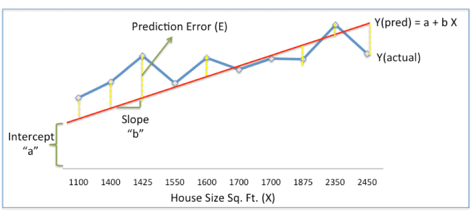
In the above chart, the red line gives the predicted house price (Ypred) given house size (X).
Ypred = a+bX
The blue line gives the actual house prices from historical data (Yactual)
The difference between Yactual and Ypred (given by the yellow dashed lines) is the prediction error (E)
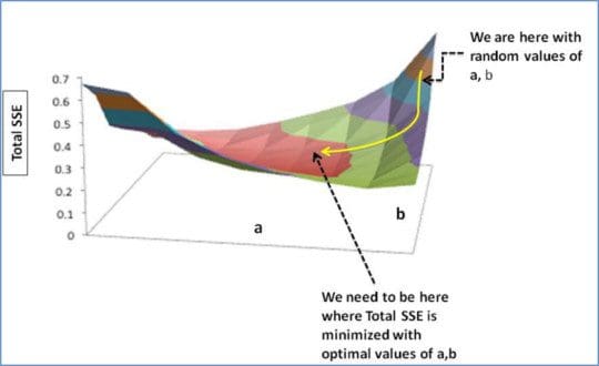
So, we need to find a line with optimal values of a,b (called weights) that best fits the historical data by reducing the prediction error and improving prediction accuracy.
So, our objective is to find optimal a, b that minimizes the error between actual and predicted values of house price (1/2 is for mathematical convenience since it helps in calculating gradients in calculus)
Sum of Squared Errors (SSE) = ½ Sum (Actual House Price – Predicted House Price)2
= ½ Sum(Y – Ypred)2
(Please note that there are other measures of Error. SSE is just one of them.)
This is where Gradient Descent comes into the picture. Gradient descent is an optimization algorithm that finds the optimal weights (a,b) that reduces prediction error.
Lets now go step by step to understand the Gradient Descent algorithm:
Step 1: Initialize the weights(a & b) with random values and calculate Error (SSE)
Step 2: Calculate the gradient i.e. change in SSE when the weights (a & b) are changed by a very small value from their original randomly initialized value. This helps us move the values of a & b in the direction in which SSE is minimized.
Step 3: Adjust the weights with the gradients to reach the optimal values where SSE is minimized
Step 4: Use the new weights for prediction and to calculate the new SSE
Step 5: Repeat steps 2 and 3 till further adjustments to weights doesn’t significantly reduce the Error
We will now go through each of the steps in detail (I worked out the steps in excel, which I have pasted below). But before that, we have to standardize the data as it makes the optimization process faster.
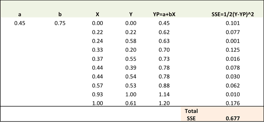
Step 1: To fit a line Ypred = a + b X, start off with random values of a and b and calculate prediction error (SSE)
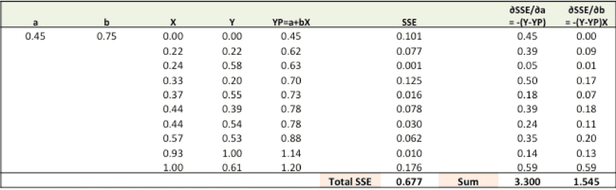
Step 2: Calculate the error gradient w.r.t the weights
∂SSE/∂a = – (Y-YP)
∂SSE/∂b = – (Y-YP)X
Here, SSE=½ (Y-YP)2 = ½(Y-(a+bX))2
You need to know a bit of calculus, but that’s about it!!
∂SSE/∂a and ∂SSE/∂b are the gradients and they give the direction of the movement of a,b w.r.t to SSE.
Step 3:Adjust the weights with the gradients to reach the optimal values where SSE is minimized
We need to update the random values of a,b so that we move in the direction of optimal a, b.
Update rules:
- a – ∂SSE/∂a
- b – ∂SSE/∂b
So, update rules:
- New a = a – r * ∂SSE/∂a = 0.45-0.01*3.300 = 0.42
- New b = b – r * ∂SSE/∂b= 0.75-0.01*1.545 = 0.73
here, r is the learning rate = 0.01, which is the pace of adjustment to the weights.
Step 4:Use new a and b for prediction and to calculate new Total SSE
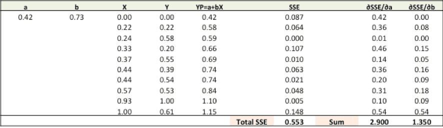
You can see with the new prediction, the total SSE has gone down (0.677 to 0.553). That means prediction accuracy has improved.
Step 5: Repeat step 3 and 4 till the time further adjustments to a, b doesn’t significantly reduces the error. At that time, we have arrived at the optimal a,b with the highest prediction accuracy.
This is the Gradient Descent Algorithm. This optimization algorithm and its variants form the core of many machine learning algorithms like Neural Networks and even Deep Learning.
Disclaimers:
Please note that this post is primarily for tutorial purposes, hence:
- The data used is fictitious and data size is extremely small. Also to simplify the example, the data and model, is a one variable example.
- This post is primarily meant to highlight how we can simplify our understanding of the math behind algorithms like Gradient descent by working them out in excel, hence there is no claim here that gradient descent gives better /worse results as compared to least square regression.
- Since the data is very small, for tutorial purposes, the entire data is being used for training. However, while building actual predictive models, various data validation techniques are leveraged (Example – Train / Test split or N- Cross Validation)
Liked what you read? To learn other algorithms in a similar simplified manner, register for the 8 week Data science course on www.deeplearningtrack.com.
Bio: Jahnavi is a machine learning and deep learning enthusiast, having led multiple machine learning teams in American Express over the last 13 years. She is the co-founder of Deeplearningtrack, an online instructor led data science training platform — www.deeplearningtrack.com
Related:
- Learning to Learn by Gradient Descent by Gradient Descent
- Getting Up Close and Personal with Algorithms
- A Concise Overview of Standard Model-fitting Methods