Ensemble Learning to Improve Machine Learning Results
Ensemble methods are meta-algorithms that combine several machine learning techniques into one predictive model in order to decrease variance (bagging), bias (boosting), or improve predictions (stacking).
By Vadim Smolyakov, Statsbot.
Ensemble learning helps improve machine learning results by combining several models. This approach allows the production of better predictive performance compared to a single model. That is why ensemble methods placed first in many prestigious machine learning competitions, such as the Netflix Competition, KDD 2009, and Kaggle.
The Statsbot team wanted to give you the advantage of this approach and asked a data scientist, Vadim Smolyakov, to dive into three basic ensemble learning techniques.
Ensemble methods are meta-algorithms that combine several machine learning techniques into one predictive model in order to decrease variance (bagging), bias (boosting), or improve predictions (stacking).
Ensemble methods can be divided into two groups:
- sequential ensemble methods where the base learners are generated sequentially (e.g. AdaBoost).
The basic motivation of sequential methods is to exploit the dependence between the base learners. The overall performance can be boosted by weighing previously mislabeled examples with higher weight. - parallel ensemble methods where the base learners are generated in parallel (e.g. Random Forest).
The basic motivation of parallel methods is to exploit independence between the base learners since the error can be reduced dramatically by averaging.
Most ensemble methods use a single base learning algorithm to produce homogeneous base learners, i.e. learners of the same type, leading to homogeneous ensembles.
There are also some methods that use heterogeneous learners, i.e. learners of different types, leading to heterogeneous ensembles. In order for ensemble methods to be more accurate than any of its individual members, the base learners have to be as accurate as possible and as diverse as possible.
Bagging
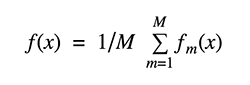
Bagging stands for bootstrap aggregation. One way to reduce the variance of an estimate is to average together multiple estimates. For example, we can train M different trees on different subsets of the data (chosen randomly with replacement) and compute the ensemble:
Bagging uses bootstrap sampling to obtain the data subsets for training the base learners. For aggregating the outputs of base learners, bagging uses voting for classification and averaging for regression.
We can study bagging in the context of classification on the Iris dataset. We can choose two base estimators: a decision tree and a k-NN classifier. Figure 1 shows the learned decision boundary of the base estimators as well as their bagging ensembles applied to the Iris dataset.
Accuracy: 0.63 (+/- 0.02) [Decision Tree]
Accuracy: 0.70 (+/- 0.02) [K-NN]
Accuracy: 0.64 (+/- 0.01) [Bagging Tree]
Accuracy: 0.59 (+/- 0.07) [Bagging K-NN]
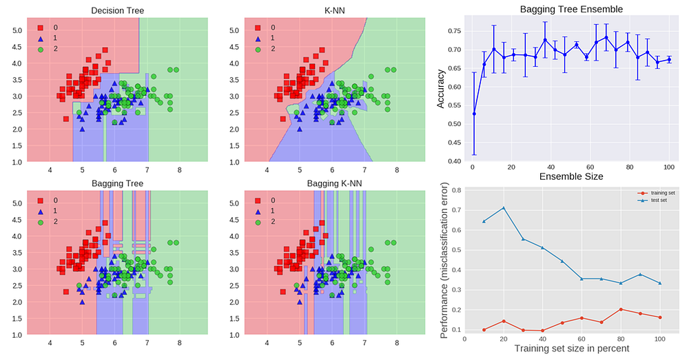
The decision tree shows the axes’ parallel boundaries, while the k=1 nearest neighbors fit closely to the data points. The bagging ensembles were trained using 10 base estimators with 0.8 subsampling of training data and 0.8 subsampling of features.
The decision tree bagging ensemble achieved higher accuracy in comparison to the k-NN bagging ensemble. K-NN are less sensitive to perturbation on training samples and therefore they are called stable learners.
Combining stable learners is less advantageous since the ensemble will not help improve generalization performance.
The figure also shows how the test accuracy improves with the size of the ensemble. Based on cross-validation results, we can see the accuracy increases until approximately 10 base estimators and then plateaus afterwards. Thus, adding base estimators beyond 10 only increases computational complexity without accuracy gains for the Iris dataset.
We can also see the learning curves for the bagging tree ensemble. Notice an average error of 0.3 on the training data and a U-shaped error curve for the testing data. The smallest gap between training and test errors occurs at around 80% of the training set size.
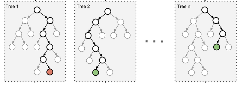
A commonly used class of ensemble algorithms are forests of randomized trees.
In random forests, each tree in the ensemble is built from a sample drawn with replacement (i.e. a bootstrap sample) from the training set. In addition, instead of using all the features, a random subset of features is selected, further randomizing the tree.
As a result, the bias of the forest increases slightly, but due to the averaging of less correlated trees, its variance decreases, resulting in an overall better model.
In an extremely randomized trees algorithm randomness goes one step further: the splitting thresholds are randomized. Instead of looking for the most discriminative threshold, thresholds are drawn at random for each candidate feature and the best of these randomly-generated thresholds is picked as the splitting rule. This usually allows reduction of the variance of the model a bit more, at the expense of a slightly greater increase in bias.
Boosting
Boosting refers to a family of algorithms that are able to convert weak learners to strong learners. The main principle of boosting is to fit a sequence of weak learners− models that are only slightly better than random guessing, such as small decision trees− to weighted versions of the data. More weight is given to examples that were misclassified by earlier rounds.
The predictions are then combined through a weighted majority vote (classification) or a weighted sum (regression) to produce the final prediction. The principal difference between boosting and the committee methods, such as bagging, is that base learners are trained in sequence on a weighted version of the data.
The algorithm below describes the most widely used form of boosting algorithm called AdaBoost, which stands for adaptive boosting.
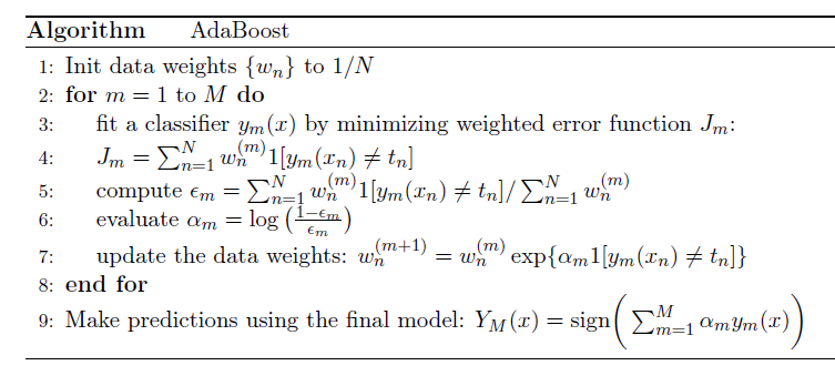
We see that the first base classifier y1(x) is trained using weighting coefficients that are all equal. In subsequent boosting rounds, the weighting coefficients are increased for data points that are misclassified and decreased for data points that are correctly classified.
The quantity epsilon represents a weighted error rate of each of the base classifiers. Therefore, the weighting coefficients alpha give greater weight to the more accurate classifiers.
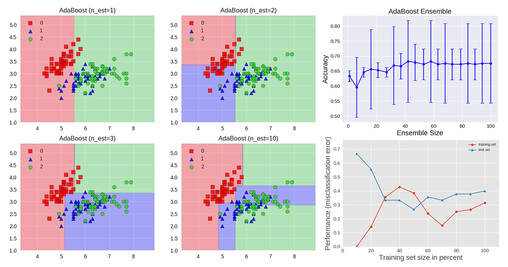
The AdaBoost algorithm is illustrated in the figure above. Each base learner consists of a decision tree with depth 1, thus classifying the data based on a feature threshold that partitions the space into two regions separated by a linear decision surface that is parallel to one of the axes. The figure also shows how the test accuracy improves with the size of the ensemble and the learning curves for training and testing data.
Gradient Tree Boosting is a generalization of boosting to arbitrary differentiable loss functions. It can be used for both regression and classification problems. Gradient Boosting builds the model in a sequential way.
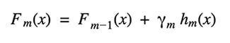
At each stage the decision tree hm(x) is chosen to minimize a loss function L given the current model Fm-1(x):
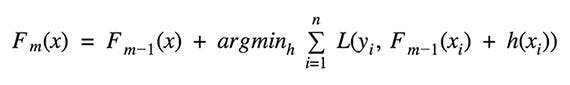
The algorithms for regression and classification differ in the type of loss function used.