A Tutorial on the Expectation Maximization (EM) Algorithm

By Elena Sharova, codefying.

We are presented with some unlabelled data and we are told that it comes from a multi-variate Gaussian distribution. Our task is to come up with the hypothesis for the means and the variances of each distribution. For example, Figure 1 shows (labelled) data drawn from two Gaussians. We need to estimate the means and variances of the x’s and the y’s of the blue and red distribution. How are we going to do this?

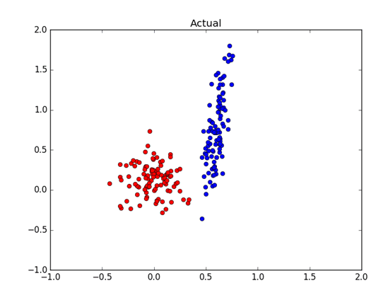
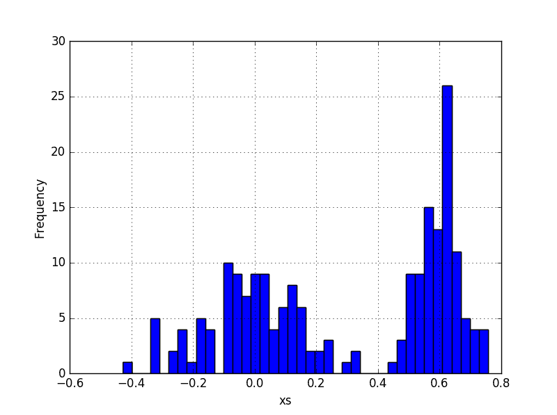
Well, we can plot the data of each dimension and estimate the means by looking at the plots. For example, we could use a histogram plot to estimate that the mean of the x’s of the blue distribution is about 0.6 and the mean of the x’s from the red distribution is about 0.0. By looking at the spread of each cluster we can estimate that the variance of blue x’s is small, perhaps 0.0, and variance of red x’s is about 0.025. That would be a pretty good guess since the actual distribution was drawn from N(0.6, 0.003) for blue and N(0.02, 0.03) for red. Can we do better than looking at the plots? Can we come up with a good estimates for the means and the variances in a more robust way?

The Expectation Maximization (EM) algorithm can be used to generate the best hypothesis for the distributional parameters of some multi-modal data. Note that we say ‘the best’ hypothesis. But what is ‘the best’? The best hypothesis for the distributional parameters is the maximum likelihood hypothesis – the one that maximizes the probability that this data we are looking at comes from K distributions, each with a mean m_k and variance sigma_k². In this tutorial we are assuming that we are dealing with K normal distributions.

In a single modal normal distribution this hypothesis h is estimated directly from the data as:

Which are simply the trusted arithmetic average and variance. In a multi-modal distribution we need to estimate h = [ m1,m2,...,mK; sigma12,sigma22,...,sigmaK2 ]. The EM algorithm is going to help us to do this. Let’s see how.

We begin with some initial estimate for each m_k~ and sigma_k²~. We will have a total of K estimates for each parameter. The estimates can be taken from the plots we made earlier, our domain knowledge, or they even can be wild (but not too wild) guesses. We then proceed to take each data point and answer the following question – what is the probability that this data point was generated from a normal distribution with mean m_k~ and sigma_k²~? That is, we repeat this question for each set of our distributional parameters. In Figure 1 we plotted data from 2 distributions. Thus we need to answer these questions twice – what is the probability that a data point x_i, i=1,...N, was drawn from N(m₁~, sigma₁²~) and what is the probability that it was drawn from N(m₂~, sigma₂²~). By the normal density function we get:

The individual probabilities only tell us half of the story because we still need to take into account the probability of picking N(m₁~, sigma₁²~) or N(m₂~, sigma₂²~) to draw the data from. We now arrive at what is known as responsibilities of each distribution for each data point. In a classification task this responsibility can be expressed as the probability that a data point x_i belongs to some class c_k:

In Equation 5 we introduce a new parameter omega_k~ which is the probability of picking k’s distribution to draw the data point from. Figure 1 indicates that each of our two clusters are equally likely to be picked. But like with m_k~ and sigma_k²~ we do not really know the value for this parameter. Therefore we need to guess it and it is a part of our hypothesis:

You could be asking yourself where the denominator in Equation 5 comes from. The denominator is the sum of probabilities of observing x_i in each cluster weighted by that cluster’s probability. Essentially, it is the total probability of observing x_i in our data.

If we are making hard cluster assignments, we will take the maximum P(x_i belongs to c_k) and assign the data point to that cluster. We repeat this probabilistic assignment for each data point. In the end this will give us the first data ‘re-shuffle’ into K clusters. We are now in a position to update the initial estimates for h to h'. These two steps of estimating the distributional parameters and updating them after probabilistic data assignments to clusters is repeated until convergences to h*. In summary, the two steps of the EM algorithm are:

1. E-step: perform probabilistic assignments of each data point to some class based on the current hypothesis h for the distributional class parameters;
2. M-step: update the hypothesis h for the distributional class parameters based on the new data assignments.

During the E-step we are calculating the expected value of cluster assignments. During the M-step we are calculating a new maximum likelihood for our hypothesis.

Bio: Elena Sharova is a data scientist, financial risk analyst and software developer. She holds an MSc in Machine Learning and Data Mining from University of Bristol.

Related:

• A comparison between PCA and hierarchical clustering
• 6 crazy things Deep Learning and Topological Data Analysis can do with your data
• Data Science 102: K-means clustering is not a free lunch