XGBoost: A Concise Technical Overview

Introduction

 

"Our single XGBoost model can get to the top three! Our final model just averaged XGBoost models with different random seeds."

- Dmitrii Tsybulevskii & Stanislav Semenov, winners of Avito Duplicate Ads Detection Kaggle competition.

With entire blogs dedicated to how the sole application of XGBoost can propel one’s ranking on Kaggle competitions, it is time we delved deeper into the concepts of XGBoost.

Bagging algorithms control for high variance in a model. However, boosting algorithms are considered more effective as they deal with both bias as well as variance (the bias-variance trade-off).

XGBoost is an implementation of Gradient Boosting Machines (GBM) and is used for supervised learning. XGBoost is an open-sourced machine learning library available in Python, R, Julia, Java, C++, Scala. The features that standout are:

1. Speed
2. Awareness of sparse data
3. Implementation on single, distributed systems and out-of-core computation
4. Parallelization

 

Working

 
In order to understand XGBoost, we must first understand Gradient Descent and Gradient Boosting.

a) Gradient Descent:

A cost function measures how close the predicted values are, to the corresponding actual values. Ideally, we want as little difference as possible between the predicted values and the actual values. Thus, we want the cost function to be minimized.

The weights associated with a trained model, cause it to predict values that are close to the actual values. Thus, the better the weights associated with the model, the more accurate are the predicted values and the lower is the cost function. With more records in the training set, the weights are learned and then updated.

Gradient Descent is an iterative optimization algorithm. It is a method to minimize a function having several variables. Thus, Gradient Descent can be used to minimize the cost function. It first runs the model with initial weights, then seeks to minimize the cost function by updating the weights over several iterations.

b) Gradient Boosting:

Boosting: An ensemble of weak learners is built, where the misclassified records are given greater weight (‘boosted’) to correctly predict them in later models. These weak learners are later combined to produce a single strong learner. There are many Boosting algorithms such as AdaBoost, Gradient Boosting and XGBoost. The latter two are tree-based models. Figure 1 depicts a Tree Ensemble Model.

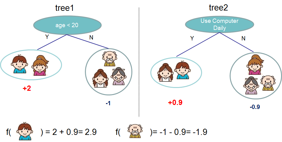
Figure 1: Tree Ensemble Model to predict whether a given user likes computer games or not. +2, +0.1, -1, +0.9, -0.9 are the prediction scores in each leaf. The final prediction for a given user is the sum of predictions from each tree. Source

Gradient Boosting carries the principle of Gradient Descent and Boosting to supervised learning. Gradient Boosted Models (GBM’s) are trees built sequentially, in series. In GBM’s, we take the weighted sum of multiple models.

• Each new model uses Gradient Descent optimization to update/ make corrections to the weights to be learned by the model to reach a local minima of the cost function.
• The vector of weights assigned to each model is not derived from the misclassifications of the previous model and the resulting increased weights assigned to misclassifications, but is derived from the weights optimized by Gradient Descent to minimize the cost function. The result of Gradient Descent is the same function of the model as the beginning, just with better parameters.
• Gradient Boosting adds a new function to the existing function in each step to predict the output. The result of Gradient Boosting is an altogether different function from the beginning, because the result is the addition of multiple functions.

c) XGBoost:

XGBoost was built to push the limit of computational resources for boosted trees. XGBoost is an implementation of GBM, with major improvements. GBM’s build trees sequentially, but XGBoost is parallelized. This makes XGBoost faster.

 

Features of XGBoost:

 
XGBoost is scalable in distributed as well as memory-limited settings. This scalability is due to several algorithmic optimizations.

1. Split finding algorithms: approximate algorithm:

To find the best split over a continuous feature, data needs to be sorted and fit entirely into memory. This may be a problem in case of large datasets.

An approximate algorithm is used for this. Candidate split points are proposed based on the percentiles of feature distribution. The continuous features are binned into buckets that are split based on the candidate split points. The best solution for candidate split points is chosen from the aggregated statistics on the buckets.

2. Column block for parallel learning:

Sorting the data is the most time-consuming aspect of tree learning. To reduce sorting costs, data is stored in in-memory units called ‘blocks’. Each block has data columns sorted by the corresponding feature value. This computation needs to be done only once before training and can be reused later.

Sorting of blocks can be done independently and can be divided between parallel threads of the CPU. The split finding can be parallelized as the collection of statistics for each column is done in parallel.

3. Weighted quantile sketch for approximate tree learning:

To propose candidate split points among weighted datasets, the Weighted Quantile Sketch algorithm is used. It carries out merge and prune operations on quantile summaries over the data.

4. Sparsity-aware algorithm:

Input may be sparse due to reasons such as one-hot encoding, missing values and zero entries. XGBoost is aware of the sparsity pattern in the data and visits only the default direction (non-missing entries) in each node.

5. Cache-aware access:

To prevent cache miss during split finding and ensure parallelization, choose 2^16 examples per block.

6. Out-of-core computation:

For data that does not fit into main memory, divide the data into multiple blocks, and store each block on the disk. Compress each block by columns and decompress on the fly by an independent thread while disk reading.

7. Regularized Learning Objective:

To measure the performance of a model given a certain set of parameters, we need to define an objective function. An objective function must always contain two parts: training loss and regularization. The regularization term penalizes the complexity of the model.

Obj(Θ)=L(θ)+ Ω(Θ)

where Ω is the regularization term which most algorithms forget to include in the objective function. However, XGBoost includes regularization, thus controlling the complexity of the model and preventing overfitting.

The above 6 features maybe individually present in some algorithms, but XGBoost combines these techniques to make an end-to-end system that provides scalability and effective resource utilization.

 

Python and R codes for implementation:

 
These links provide a good start to implement XGBoost using Python and R.

The following XGBoost code in Python works on the Pima Indians Diabetes dataset. It predicts whether diabetes will occur or not in patients of Pima Indian heritage. This code is inspired from tutorials by Jason Brownlee.

 

Conclusion

 
You can refer to this paper, written by the developers of XGBoost, to learn of its detailed working. You can also find the project on Github and view tutorials and usecases here.

XGBoost however, should not be used as a silver bullet. Best results can be obtained in conjunction with great data exploration and feature engineering.

 
Related:

• XGBoost, a top Machine Learning method on Kaggle, Explained
• XGBoost, Implementing the Winningest Kaggle algortithm in Spark and Flink
• A simple XGBoost tutorial using the Iris dataset