


Building an Audio Classifier using Deep Neural Networks
Using a deep convolutional neural network architecture to classify audio and how to effectively use transfer learning and data-augmentation to improve model accuracy using small datasets.
Understanding sound is one of the basic tasks that our brain performs. This can be broadly classified into Speech and Non-Speech sounds. We have noise robust speech recognition systems in place but there is still no general purpose acoustic scene classifier which can enable a computer to listen and interpret everyday sounds and take actions based on those like humans do, like moving out of the way when we listen to a horn or hear a dog barking behind us etc.
Our model is only as complex as our data, thus getting labelled ‘data is very important in machine learning’. The complexity of the Machine Learning systems arise from the data itself and not from the algorithms. In the past few years we’ve seen deep learning systems take over the field of image recognition and captioning, with architectures like ResNet, GoogleNet shattering benchmarks in the ImageNet competition with 1000 categories of images, classified at above 95% accuracy (top 5 accuracy). This was due to a large amount of labelled dataset that were available for the Models to train on and also faster computers with GPU acceleration which makes it easier to train Deep Models.
The problem we face with building a noise robust acoustic classifier is the lack of a large dataset, but Google recently launched the AudioSet - which is a large collection of labelled audio taken from YouTube videos (10s excerpts). Earlier, we had the ESC-50 dataset with 2000 recordings, 40 from each class covering many everyday sounds.
Step 1. Extracting Features
Although deep learning eliminates the need for hand-engineered features, we have to choose a representation model for our data. Instead of directly using the sound file as an amplitude vs time signal we use a log-scaled mel-spectrogram with 128 components (bands) covering the audible frequency range (0-22050 Hz), using a window size of 23 ms (1024 samples at 44.1 kHz) and a hop size of the same duration. This conversion takes into account the fact that human ear hears sound on log-scale, and closely scaled frequency are not well distinguished by the human Cochlea. The effect becomes stronger as frequency increases. Hence we only take into account power in different frequency bands. This sample code gives an insight into converting audio files into spectrogram images. We use glob and librosa library - this code is a standard one for conversion into spectrogram and you’re free to make modifications to suit the needs.
In the code that follows,
parent_dir = string with name of main directory.
sub_dirs = a list of directories inside parent we want to explore
So all *.wav files in the area parent_dir/sub_dirs/*.wav are extracted, iterating through all subdirs.
There is an interesting article about mel-scale and mfcc coefficients for people who are interested. Ref.
Now the audio file is represented as a 128(frames) x 128(bands) spectrogram image.

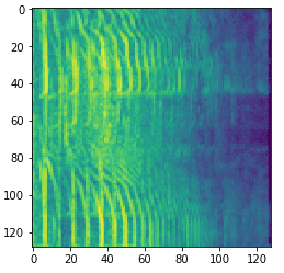
The Audio-classification problem is now transformed into an image classification problem. We need to detect presence of a particular entity ( ‘Dog’,’Cat’,’Car’ etc) in this image.
Step 2. Choosing an Architecture
We use a convolutional Neural Network, to classify the spectrogram images.This is because CNNs work better in detecting local feature patterns (edges etc) in different parts of the image and are also good at capturing hierarchical features which become subsequently complex with every layer as illustrated in the image

Another way to think about this is to use a Recurrent Neural Network to capture the sequential information in sound data by passing one frame at a time, but as in most cases CNNs have outperformed standalone RNNs - we haven’t used it in this particular experiment. In many cases RNNs are used along with CNNs to improve performance of networks and we would be experimenting with those architectures in the future. [Ref]
Step 3. Transfer Learning
As the CNNs learn features hierarchically, we can observe that the initial few layers learn basic features like various edges which are common to many different types of images. Transfer learning is the concept of training the model on a dataset with large amounts of similar data and then modifying the network to perform well on the target task where we do not have a lot of data. This is also called fine-tuning - this blog explains transfer learning very well.
Step 4. Data Augmentation
While dealing with small datasets, learning complex representations of the data is very prone to overfitting as the model just memorises the dataset and fails to generalise. One way to beat this is to augment the audio files into producing many files each with a slight variation.
The ones we used here are time-stretching and pitch-shifting - Rubberband is an easy to use library for this purpose.
rubberband -t 1.5 -p 2 input.wav output.wav
This one line terminal command, gives us a new audio file which is 50% longer than original and has pitch shifted up by one octave.
To visualise what this means, look at this image of a cat I took from the internet.
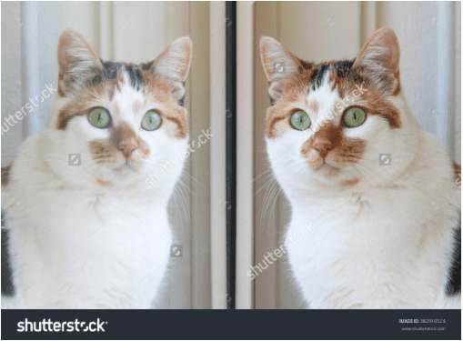
If we only have the image on our right, we can use data augmentation to make a mirror image of that image and it’s still a cat (Additional training data!). For a computer these are two completely different pixel distributions and helps it learn more general concepts (if A is a dog, mirror image of A is dog too).
Similarly we apply time-stretching (either slow down the sound or speed it up) , and
pitch-shifting (make it more or less shrill) to get more generalised training data for our network (also improved the validation accuracy by 8-9% in this case due to a small training set).
We observed that the performance of the model for each sound class is influenced differently by each augmentation set, suggesting that the performance of the model could be improved further by applying class-conditional data augmentation.
Overfitting is a major problem in the field of deep learning and we can use Data Augmentation as one way to combat this problem , other ways of implicitly generalising include using dropout layers and L1,L2 regularisation. [Ref]
So in this article we proposed a deep convolutional neural network architecture which helps us classify audio and how to effectively use transfer learning and data-augmentation to improve model accuracy in case of small datasets.
Bio: Narayan Srinivasan is interested in building autonomous vehicle. He is a graduate of Indian Institute of Technology, Madras.
Related