The 10 Deep Learning Methods AI Practitioners Need to Apply

comments

Interest in machine learning has exploded over the past decade. You see machine learning in computer science programs, industry conferences, and the Wall Street Journal almost daily. For all the talk about machine learning, many conflate what it can do with what they wish it could do. Fundamentally, machine learning is using algorithms to extract information from raw data and represent it in some type of model. We use this model to infer things about other data we have not yet modeled.

Neural networks are one type of model for machine learning; they have been around for at least 50 years. The fundamental unit of a neural network is a node, which is loosely based on the biological neuron in the mammalian brain. The connections between neurons are also modeled on biological brains, as is the way these connections develop over time (with “training”).

In the mid-1980s and early 1990s, many important architectural advancements were made in neural networks. However, the amount of time and data needed to get good results slowed adoption, and thus interest cooled. In the early 2000s, computational power expanded exponentially and the industry saw a “Cambrian explosion” of computational techniques that were not possible prior to this. Deep learning emerged from that decade’s explosive computational growth as a serious contender in the field, winning many important machine learning competitions. The interest has not cooled as of 2017; today, we see deep learning mentioned in every corner of machine learning.

To get myself into the craze, I took Udacity’s “Deep Learning” course, which is a great introduction to the motivation of deep learning and the design of intelligent systems that learn from complex and/or large-scale datasets in TensorFlow. For the class projects, I used and developed neural networks for image recognition with convolutions, natural language processing with embeddings and character based text generation with Recurrent Neural Network / Long Short-Term Memory. All the code in Jupiter Notebook can be found on this GitHub repository.

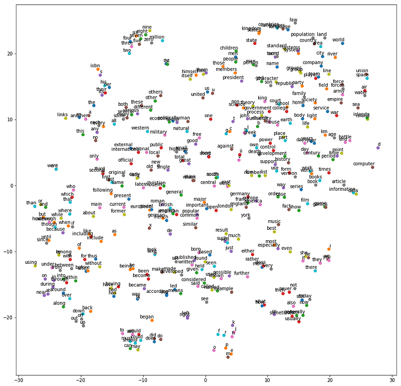
Here is an outcome of one of the assignments, a t-SNE projection of word vectors, clustered by similarity.

Most recently, I have started reading academic papers on the subject. From my research, here are several publications that have been hugely influential to the development of the field:

• NYU’s Gradient-Based Learning Applied to Document Recognition (1998), which introduces Convolutional Neural Network to the Machine Learning world.
• Toronto’s Deep Boltzmann Machines (2009), which presents a new learning algorithm for Boltzmann machines that contain many layers of hidden variables.
• Stanford & Google’s Building High-Level Features Using Large-Scale Unsupervised Learning (2012), which addresses the problem of building high-level, class-specific feature detectors from only unlabeled data.
• Berkeley’s DeCAF — A Deep Convolutional Activation Feature for Generic Visual Recognition (2013), which releases DeCAF, an open-source implementation of the deep convolutional activation features, along with all associated network parameters to enable vision researchers to be able to conduct experimentation with deep representations across a range of visual concept learning paradigms.
• DeepMind’s Playing Atari with Deep Reinforcement Learning (2016), which presents the 1st deep learning model to successfully learn control policies directly from high-dimensional sensory input using reinforcement learning.

There is an abundant amount of great knowledge about deep learning I have learnt via research and learning. Here I want to share the 10 powerful deep learning methods AI engineers can apply to their machine learning problems. But first of all, let’s define what deep learning is. Deep learning has been a challenge to define for many because it has changed forms slowly over the past decade. To set deep learning in context visually, the figure below illustrates the conception of the relationship between AI, machine learning, and deep learning.

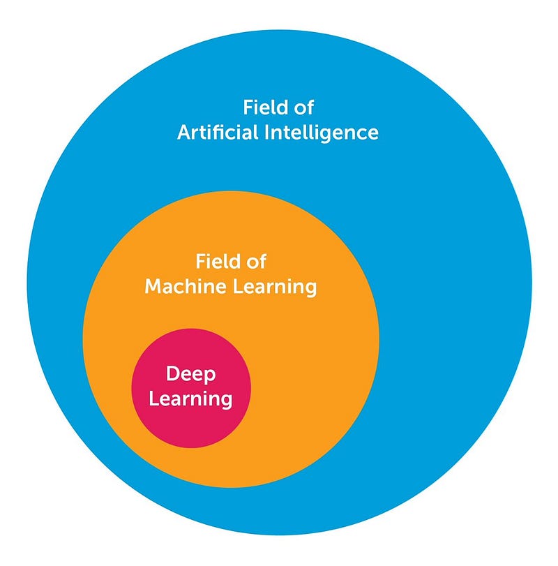
The field of AI is broad and has been around for a long time. Deep learning is a subset of the field of machine learning, which is a subfield of AI. The facets that differentiate deep learning networks in general from “canonical” feed-forward multilayer networks are as follows:

• More neurons than previous networks
• More complex ways of connecting layers
• “Cambrian explosion” of computing power to train
• Automatic feature extraction

When I say “more neurons”, I mean that the neuron count has risen over the years to express more complex models. Layers also have evolved from each layer being fully connected in multilayer networks to locally connected patches of neurons between layers in Convolutional Neural Networks and recurrent connections to the same neuron in Recurrent Neural Networks (in addition to the connections from the previous layer).
Deep learning then can be defined as neural networks with a large number of parameters and layers in one of four fundamental network architectures:

• Unsupervised Pre-trained Networks
• Convolutional Neural Networks
• Recurrent Neural Networks
• Recursive Neural Networks

In this post, I am mainly interested in the latter 3 architectures. A Convolutional Neural Network is basically a standard neural network that has been extended across space using shared weights. CNN is designed to recognize images by having convolutions inside, which see the edges of an object recognized on the image. A Recurrent Neural Network is basically a standard neural network that has been extended across time by having edges which feed into the next time step instead of into the next layer in the same time step. RNN is designed to recognize sequences, for example, a speech signal or a text. It has cycles inside that implies the presence of short memory in the net. A Recursive Neural Network is more like a hierarchical network where there is really no time aspect to the input sequence but the input has to be processed hierarchically in a tree fashion. The 10 methods below can be applied to all of these architectures.

1 — Back-Propagation

Back-prop is simply a method to compute the partial derivatives (or gradient) of a function, which has the form as a function composition (as in Neural Nets). When you solve an optimization problem using a gradient-based method (gradient descent is just one of them), you want to compute the function gradient at each iteration.

For a Neural Nets, the objective function has the form of a composition. How do you compute the gradient? There are 2 common ways to do it: (i) Analytic differentiation. You know the form of the function. You just compute the derivatives using the chain rule (basic calculus). (ii) Approximate differentiation using finite difference. This method is computationally expensive because the number of function evaluation is O(N), where N is the number of parameters. This is expensive, compared to analytic differentiation. Finite difference, however, is commonly used to validate a back-prop implementation when debugging.

2 — Stochastic Gradient Descent

An intuitive way to think of Gradient Descent is to imagine the path of a river originating from top of a mountain. The goal of gradient descent is exactly what the river strives to achieve — namely, reach the bottom most point (at the foothill) climbing down from the mountain.

Now, if the terrain of the mountain is shaped in such a way that the river doesn’t have to stop anywhere completely before arriving at its final destination (which is the lowest point at the foothill, then this is the ideal case we desire. In Machine Learning, this amounts to saying, we have found the global mimimum (or optimum) of the solution starting from the initial point (top of the hill). However, it could be that the nature of terrain forces several pits in the path of the river, which could force the river to get trapped and stagnate. In Machine Learning terms, such pits are termed as local minima solutions, which is not desirable. There are a bunch of ways to get out of this (which I am not discussing).

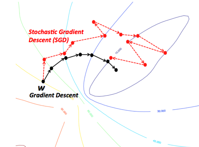
Gradient Descent therefore is prone to be stuck in local minimum, depending on the nature of the terrain (or function in ML terms). But, when you have a special kind of mountain terrain (which is shaped like a bowl, in ML terms this is called a Convex Function), the algorithm is always guaranteed to find the optimum. You can visualize this picturing a river again. These kind of special terrains (a.k.a convex functions) are always a blessing for optimization in ML. Also, depending on where at the top of the mountain you initial start from (ie. initial values of the function), you might end up following a different path. Similarly, depending on the speed at the river climbs down (ie. the learning rate or step size for the gradient descent algorithm), you might arrive at the final destination in a different manner. Both of these criteria can affect whether you fall into a pit (local minima) or are able to avoid it.

3 — Learning Rate Decay

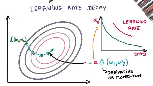
Adapting the learning rate for your stochastic gradient descent optimization procedure can increase performance and reduce training time. Sometimes this is called learning rate annealing or adaptive learning rates. The simplest and perhaps most used adaptation of learning rate during training are techniques that reduce the learning rate over time. These have the benefit of making large changes at the beginning of the training procedure when larger learning rate values are used, and decreasing the learning rate such that a smaller rate and therefore smaller training updates are made to weights later in the training procedure. This has the effect of quickly learning good weights early and fine tuning them later.

Two popular and easy to use learning rate decay are as follows:

• Decrease the learning rate gradually based on the epoch.
• Decrease the learning rate using punctuated large drops at specific epochs.