Exploring Recurrent Neural Networks

comments

By Packtpub.

In this tutorial, taken from Hands-on Deep Learning with Theano by Dan Van Boxel, we’ll be exploring recurrent neural networks. We’ll start off by looking at the basics, before looking at RNNs through a motivating weather modeling problem. We’ll also implement and train an RNN in TensorFlow.

In a typical model, you have some X input features and some Y output you want to predict. We usually consider our different training samples as independent observations. So, the features from data point one shouldn't impact the prediction for data point two. But what if our data points are correlated? The most common example is that each data point, Xt, represents features collected at time t. It's natural to suppose that the features at time t and time t+1 will both be important to the prediction at time t+1. In other words, history matters.

Now, when modeling, you could just include twice as many input features, adding the previous time step to the current ones, and computing twice as many input weights. But, if you're going through all the effort of building a neural network to compute transform features, it would be nice if you could use the intermediate features from the previous time step, in the current time step network.

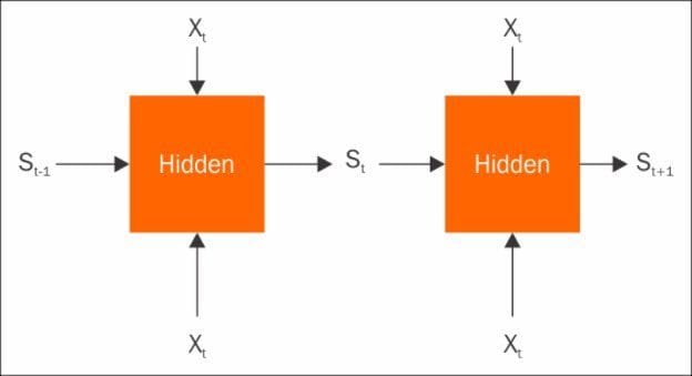
RNNs do exactly this. Consider your input, Xt as usual, but add in some state, St-1 that comes from the previous time step, as additional features. Now you can compute weights as usual to predict Yt, and you produce a new internal state, St, to be used in the next time step. For the first time step, it's typical to use a default or zero initial state. Classic RNNs are literally this simple, but there are more advanced structures common in literature today, such as gated recurrent units and long short-term memory circuits. These are beyond the scope of this tutorial, but work on the same principles and generally apply to the same types of problems.

Modeling the weights

You might be wondering how we'll compute weights with all these dependents on the previous time step. Computing the gradients does involve recursing back through the time computation, but fear not, TensorFlow handles the tedious stuff and let's us do the modeling:

# read in data
filename = 'weather.npz'
data = np.load(filename)
daily = data['daily']
weekly = data['weekly']

num_weeks = len(weekly)
dates = np.array([datetime.datetime.strptime(str(int(d)),
        '%Y%m%d') for d in weekly[:,0]])

To use RNNs, we need a data modeling problem with a time component.

The font classification problem isn't really appropriate here. So, let's take a look at some weather data. The weather.npz file is a collection of weather station data from a city in the United States over several decades. The daily array contains measurements from every day of the year. There are six columns to the data, starting with the date. Next, is the precipitation, measuring any rainfall in inches that day. After this, come two columns for snow—the first is measured snow currently on the ground, while the latter is snowfall on that day, again, in inches. Finally, we have some temperature information, the daily high and the daily low in degrees Fahrenheit.

The weekly array, which we'll use, is a weekly summary of the daily information. We'll use the middle date to indicate the week, then, we'll sum up all rainfall for the week. For snow, however, we'll average the snow on the ground, since it doesn't make sense to add snow from one cold day to the same snow sitting on the ground the next day. Snowfall though, we'll total for the week, just like rain. Finally, we'll average the high and low temperatures for the week respectively. Now that you've got a handle on the dataset, what shall we do with it? One interesting time-based modeling problem would be trying to predict the season of a particular week using it's weather information and the history of previous weeks.

In the Northern Hemisphere, in the United States, it's warmer during the months of June through August and colder during December through February, with transitions in between. Spring months tend to be rainy, and winter often includes snow. While one week can be highly variable, a history of weeks should provide some predictive power.

Understanding RNNs

First, let's read in the data from a compressed NumPy array. The weather.npz file happens to include the daily data as well, if you wish to explore your own model; np.load reads both arrays into a dictionary and will set weekly to be our data of interest; num_weeks is naturally how many data points we have, here, several decades worth of information:

num_weeks = len(weekly)

To format the weeks, we use a Python datetime.datetime object reading the storage string in year month day format:

dates = np.array([datetime.datetime.strptime(str(int(d)),
        '%Y%m%d') for d in weekly[:,0]])

We can use the date of each week to assign its season. For this model, because we're looking at weather data, we use the meteorological season rather than the common astronomical season. Thankfully, this is easy to implement with the Python function. Grab the month from the datetime object and we can directly compute this season. Spring, season zero, is March through May, summer is June through August, autumn is September through November, and finally, winter is December through February. The following is the simple function that just evaluates the month and implements that:

def assign_season(date):
  ''' Assign season based on meteorological season.
      Spring - from Mar 1 to May 31
      Summer - from Jun 1 to Aug 31
      Autumn - from Sep 1 to Nov 30
      Winter - from Dec 1 to Feb 28 (Feb 29 in a leap year)
  '''
  month = date.month
  # spring = 0
  if 3 <= month < 6:
     season = 0
  # summer = 1
  elif 6 <= month < 9:
    season = 1
  # autumn = 2
  elif 9 <= month < 12:
    season = 2
  # winter = 3
  elif month == 12 or month < 3:
    season = 3
  return season

Let's note that we have four seasons and five input variables and, say, 11 values in our history state:

# There are 4 seasons
num_classes = 4

# and 5 variables
num_inputs = 5

# And a state of 11 numbers
state_size = 11

Now you're ready to compute the labels:

labels = np.zeros([num_weeks,num_classes])

# read and convert to one-hot

for i,d in enumerate(dates):

labels[i,assign_season(d)] = 1

We do this directly in one-hot format, by making an all-zeroes array and putting a one in the position of the assign season.

Cool! You just summarized decades of time with a few commands.

As these input features measure very different things, namely rainfall, snow, and temperature, on very different scales, we should take care to put them all on the same scale. In the following code, we grab the input features, skipping the date column of course, and subtract the average to center all features at zero:

# extract and scale training data

train = weekly[:,1:]

train = train - np.average(train,axis=0)

train = train / train.std(axis=0)

Then, we scale each feature by dividing by its standard deviation. This accounts for temperatures ranging roughly 0 to 100, while rainfall only changes between about 0 and 10. Nice work on the data prep! It isn't always fun, but it's a key part of machine learning and TensorFlow.

Let's now jump into the TensorFlow model:

# These will be inputs

x = tf.placeholder("float", [None, num_inputs])

# TF likes a funky input to RNN

x_ = tf.reshape(x, [1, num_weeks, num_inputs])

We input our data as normal with a placeholder variable, but then you see this strange reshaping of the entire data set into one big tensor. Don't worry, this is because we technically have one long, unbroken sequence of observations. The y_ variable is just our output:

y_ = tf.placeholder("float", [None,num_classes])

We'll be computing a probability for every week for each season.

The cell variable is the key to the recurrent neural network:

cell = tf.nn.rnn_cell.BasicRNNCell(state_size)

This tells TensorFlow how the current time step depends on the previous. In this case, we'll use a basic RNN cell. So, we're only looking back one week at a time. Suppose that it has state size or 11 values. Feel free to experiment with more exotic cells and different state sizes.

To put that cell to use, we'll use tf.nn.dynamic_rnn:

outputs, states = tf.nn.dynamic_rnn(cell,x_,

dtype=tf.nn.dtypes.float32, initial_state=None)

This intelligently handles the recursion rather than simply unrolling all the time steps into a giant computational graph. As we have thousands of observations in one sequence, this is critical to attain reasonable speed. After the cell, we specify our input x_, then dtype to use 32 bits to store decimal numbers in a float, and then the empty initial_state. We use the outputs from this to build a simple model. From this point on, the model is almost exactly as you would expect from any neural network:

We'll multiply the output of the RNN cells, some weights, and add a bias to get a score for each class for that week:

W1 = tf.Variable(tf.truncated_normal([state_size,num_classes],
        stddev=1./math.sqrt(num_inputs)))

b1 = tf.Variable(tf.constant(0.1,shape=[num_classes]))

# reshape the output for traditional usage
h1 = tf.reshape(outputs,[-1,state_size])

Our categorical cross_entropy loss function and train optimizer should be very familiar to you:

# Climb on cross-entropy
cross_entropy = tf.reduce_mean(tf.nn.softmax_cross_entropy_with_logits(y + 1e-50, y_))

# How we train
train_step = tf.train.GradientDescentOptimizer(0.01).minimize(cross_entropy)

# Define accuracy
correct_prediction = tf.equal(tf.argmax(y,1),tf.argmax(y_,1))
accuracy=tf.reduce_mean(tf.cast(correct_prediction, "float"))

Great work setting up the TensorFlow model! To train this, we'll use a familiar loop:

# Actually train
epochs = 100
train_acc = np.zeros(epochs//10)

for i in tqdm(range(epochs), ascii=True):
    if i % 10 == 0:

   # Record summary data, and the accuracy
     # Check accuracy on train set 
     A = accuracy.eval(feed_dict={x: train, y_: labels})
     train_acc[i//10] = A

   train_step.run(feed_dict={x: train, y_: labels})

Since this is a fictitious problem, we'll not worry too much about how accurate the model really is. The goal here is just to see how an RNN works. You can see that it runs just like any TensorFlow model:

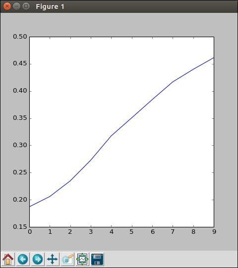
If you do look at the accuracy, you can see that it's doing pretty well; much better than the 25 percent random guessing, but still has a lot to learn.

We hope you enjoyed this extract from Hands On Deep Learning with TensorFlow. If you’d like to learn more visit packtpub.com.

Related:

• A Guide For Time Series Prediction Using Recurrent Neural Networks (LSTMs)
• Going deeper with recurrent networks: Sequence to Bag of Words Model
• 7 Steps to Mastering Deep Learning with Keras