Deep Learning in H2O using R
This article is about implementing Deep Learning (DL) using the H2O package in R. We start with a background on DL, followed by some features of H2O's DL framework, followed by an implementation using R.
 This article is about implementing Deep Learning using the H2O package in R.
H2O is an open-source Artificial Intelligence platform that allows us to use Machine Learning techniques such as Naïve Bayes, K-means, PCA, Deep Learning, Autoencoders using Deep Learning, among others. Using H2O, we can build predictive models using programming environments such as R, Python, Scala and a web-based UI called Flow.
I. Deep Learning: A Background
(Source)
Deep Learning is a branch of Machine Learning algorithms that are inspired by the functioning of the human brain and the nervous system. The input data is clamped to the input layer of the deep network. The network then uses a hierarchy of hidden layers that successively produce compact, higher level abstractions (representations) of the input data. It thus produces pseudo-features of the input features. Neural networks with 3 layers or more are considered ‘Deep’.
As an example, for the task of face detection, the raw input is usually a vector of pixel values. The first abstraction may identify pixels of light and shade; the second abstraction may identify edges and shapes; the third abstraction may put together these edges and shapes to form parts such as the eyes, nose; the next abstraction may put these parts together to form a face. Thus, complex representations are learnt using the composition of simpler representations.
At the output layer, the network error (cost) is calculated. This cost is successively minimized using a method called stochastic gradient descent and propagated backwards, back to the input layer, using an algorithm called backpropagation. This causes a re-calibration of the weights and biases in the network. Using the new weights, newer representations are propagated forward to the output layer and again checked for the network error. The process of forward and backward propagation continues until the weights have been adjusted to accurately predict the output.
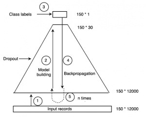
Figure 1: Pyramid illustrating Deep Learning (Source)
For Figure 1, let us consider an input dataset of 150 * 12000 dimensions (150 rows, 12000 columns). We create a Deep network with 4 hidden layers consisting of 4000, 750, 200, 30 neurons. All the 12000 data points in the input layer are used to construct the 4000 pseudo-features of the first hidden layer. As the size of the network here progressively decreases towards the final hidden layer, it forms a pyramid. The 5 steps shown in the figure have been explained below.
Step 1: Feed the input records (150* 12000) into the network.
Step 2: The Deep Learning algorithm begins to learn inherent patterns in the dataset. It does so by associating a weight and bias to every feature formed from the input layer and hidden layers. This is the model-building stage. As it passes through each successive hidden layer, it forms narrower abstractions of the data. Each abstraction takes the abstraction of the previous layer as its input.
Dropout is a hyper-parameter specified during the model-building stage.
Step 3: After passing through the last hidden layer here, an abstraction of 150* 30 features is formed. The class labels (150* 1) are exposed to this abstraction. It has been a feedforward neural network so far.
Step 4: The class labels help the model associate an outcome to the patterns created for every input record. Accordingly, now the weights and biases can be tuned to better match the labels and minimize the cost (difference between the predicted output and actual output for the record).
Stochastic Gradient Descent uses random training set samples iteratively to minimize the cost. This is done by going backwards from the output layer towards the input layer and is called backpropagation. Backpropagation trains deep networks, using the algorithm of Stochastic Gradient Descent.
Step 5: Backpropagation occurs n times, where n = number of epochs, or until there is no change in the weights.
II. Deep Learning in H2O:
Deep Learning in H2O is implemented natively as a Multi-Layer Perceptron (MLP). But, H2O also allows us to build autoencoders (an autoencoder is a neural net that takes a set of inputs, compresses and encodes them, and then tries to reconstruct the input as accurately as possible). Recurrent Neural Networks and Convolutional Neural Networks can be constructed using H2O’s Deep Water Project through third-party integrations of other Deep Learning libraries such as Caffe and TensorFlow.
The user has to specify the values of the hyper-parameters of the Deep Learning model. Parameters refer to the weights and biases of a deep learning model. Hyper-parameters are the options one needs to design a neural net, like number of layers, nodes per layer, activation, choice of regularizer, among others.
The computations of the global model parameters can be run on a single node or a multi-node cluster. For a multi-node cluster, a copy of the global model parameters is trained on the local data of a compute node, through multi-threaded and distributed parallel computation. The model is averaged across the network with each compute node contributing periodically to the global model.
Some of the features of H2O’s Deep Learning models are:
1) Automatic ‘adaptive learning rate:
ADADELTA algorithm’(‘adaptive_rate’ hyper-parameter) for faster convergence and reduced oscillation around ravines, optional value of slower learning rate called ‘rate_annealing’ to slow down the learning rate as the model approaches a minima in the optimization landscape.
2) Model regularization:
To avoid overfitting, H2O’s Deep Learning uses l1 and l2 regularization; and the concept of ‘dropouts’.
- l1 : l1 constrains the absolute value of the weights. It causes many weights to become 0.
- l2: l2 constrains the sum of the squared weights. It causes many weights to become small.
- input_dropout_ratio: input_dropout_ratio refers to the fraction of features to be dropped out / omitted from each training record, in order to improve generalization. As an example, ‘ input_dropout_ratio = 0.1’ means 10% of input features are being dropped.
- hidden_dropout_ratios: hidden_dropout_ratios refers to the fraction of features to be dropped out / omitted from each hidden layer, in order to improve generalization. As an example, ‘ hidden_dropout_ratios = c( 0.1, 0.1)’ means 10% of hidden features are dropped in each hidden layer, in a DL model having 2 hidden layers.
3) Model checkpointing:
Checkpointing (using its key= ‘model_id’) is used to resume the training of the saved previous model with more data, changed values of hyper-parameters and so forth.
4) Grid Search:
In order to compare the performance of models and tune the values of hyper-parameters, a Grid Search model trains all possible models obtained by combining sets of hyper-parameters.
The example below (source) shows 3 different topologies of hidden layers and the number of neurons, 2 different values of l1 regularization. Thus, the model Model_Grid1 trains 6 different models.
5) H2O also allows to perform Cross-validation on the training_frame and can also implement the GBM method (Gradient Boosting Machine).
III. Common R Commands for Deep Learning:
From this source:
- library(h2o): Imports the H2O R package.
- h2o.init(): Connects to (or starts) an H2O cluster.
- h2o.shutdown(): Shuts down the H2O cluster.
- h2o.importFile(path): Imports a file into H2O.
- h2o.deeplearning(x,y,training frame,hidden,epochs): Creates a Deep Learning model.
- h2o.grid(algorithm,grid id,...,hyper params = list()): Starts H2O grid support and gives results.
- h2o.predict(model, newdata): Generate predictions from an H2O model on a test set.
IV. R Script:
I have used the UCI Machine Learning 'Pima Indians' dataset.
Related:
- Deep Learning for Internet of Things Using H2O
- Decision Boundaries for Deep Learning and other Machine Learning classifiers
- Interview: Arno Candel, H20.ai on How to quick start Deep Learning with H2O