 Logistic Regression: A Concise Technical Overview
 Logistic Regression: A Concise Technical Overview
Interested in learning the concepts behind Logistic Regression (LogR)? Looking for a concise introduction to LogR? This article is for you. Includes a Python implementation and links to an R script as well.
I. Introduction:
A popular statistical technique to predict binomial outcomes (y = 0 or 1) is Logistic Regression. Logistic regression predicts categorical outcomes (binomial / multinomial values of y), whereas linear Regression is good for predicting continuous-valued outcomes (such as weight of a person in kg, the amount of rainfall in cm).
The predictions of Logistic Regression (henceforth, LogR in this article) are in the form of probabilities of an event occurring, ie the probability of y=1, given certain values of input variables x. Thus, the results of LogR range between 0-1.
LogR models the data points using the standard logistic function, which is an S- shaped curve given by the equation:
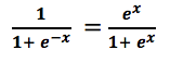
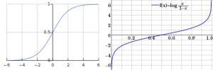
Figure 1: (Left): Standard Logistic function :Source | (Right): Logit function :Source
As shown in Figure1, the logit function on the right- with a range of - ∞ to +∞, is the inverse of the logistic function shown on the left- with a range of 0 to 1.
II. Concepts:
The equation to be solved in LogR is:
![]()
where:
- p = probability that y=1 given the values of the input features, x.
- x1,x2,..,xk = set of input features, x.
- B0,B1,..,Bk = parameter values to be estimated via the maximum likelihood method. B0,B1,..Bk are estimated as the ‘log-odds’ of a unit change in the input feature it is associated with.
- Bt = vector of coefficients
- X = vector of input features
Estimating the values of B0,B1,..,Bk involves the concepts of probability, odds and log odds. Let us note their ranges first:
- Probability ranges from 0 to 1
- Odds range from 0 to ∞
- Log odds range from -∞ to +∞
EXAMPLE:
The example dataset here is sourced from the UCLA website.
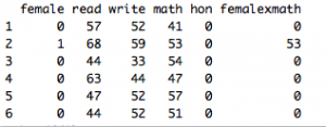
The task is to predict which students graduated with honours or not (y = 1 or 0), for 200 students with fields female, read, write, math, hon, femalexmath . The fields describe the gender (female=1 if female), reading scores, writing scores, math scores, honours status (hon=1 if graduated with honours) and femalexmath showing the math score if female=1.
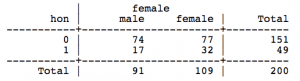
The crosstab of the variable hon with female shows that there are 109 males and 91 females; 32 of those 109 females secured honours.
Probability:
The probability of an event is the number of instances of that event divided by the total number of instances present.
Thus, the probability of females securing honours:
![]()
= 32/ 109
= 0.29
Odds:
The odds of an event is the probability of that event occurring (probability that y=1), divided by the probability that it does not occur.
Thus, the odds of females securing honours:
![]()
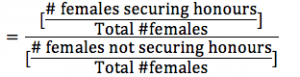
![]()
= 32/77
= 0.4155
≈ 0.42
This is interpreted as:
- 32/77 => For every 32 females that secure honours, there are 77 females that do not secure honours.
- 32/77 => There are 32 females that secure honours, for every 109 (ie 32+77) females.
Log odds:
The Logit or log-odds of an event is the log of the odds. This refers to the natural log (base ‘e’). Thus,
![]()
Thus, the log-odds of females securing honours:
![]()
Odds ratio:
It is the ratio of 2 odds; these 2 odds are obtained at 2 different values of x, the 2 values of x being 1 unit apart.
Such as: The odds obtained when x=0 and x=1 (ie when there is a 1 unit change in the value of x, where x=0 denotes male and x=1 denotes female).
Q: Find the odds ratio of graduating with honours for females and males.

=> As OR= 1.82, the odds for females graduating with honours is about 82% higher than the odds for males graduating with honours.
III. Calculations for probability:
Suppose we want to calculate the effect of being female on the probability of graduating with honours.
![]()
Where :
- B0,B1,..Bk are estimated as the ‘log-odds’ of a unit change in the input feature it is associated with.
- As B0 is the coefficient not associated with any input feature, B0= log-odds of the reference variable, x=0 (ie x=male). ie Here, B0= log[odds(male graduating with honours)]
- As B1 is the coefficient of the input feature ‘female’,
- B1= log-odds obtained with a unit change in x= female.
- B1= log-odds obtained when x=female and x=male.

Calculations:
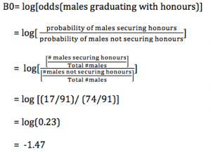
![]()
From the calculation in the section ‘odds ratio(OR)’,
B1= log (1.82)
B1= 0.593
Thus, the LogR equation becomes
y= -1.47 + 0.593* female
where the value of female is substituted as 0 or 1 for male and female respectively.
Now, let us try to find out the probability of a female securing honours when there is only 1 input feature present-‘female’.
Substitute female=1 in: y= -1.47 + 0.593* female
Thus, y=log[odds(female)]= -1.47 + 0.593*1 = -0.877
- As log-odds = -0.877.
- Thus, odds= e^ (Bt.X)= e^ (-0.877)= 0.416
- And, probability is calculated as:

Thus, the probability of a female securing honours when there is only 1 input feature present-‘female’, is 0.29.
Thus, methodology of LogR:
- To find the values of coefficents B0, B1, B2,…Bk to plug into the equation: y= log(p/(1-p))= β0 + β1*x1 + … + βk*xk = Bt.X , for specific values of x.
- The result of substituting the values of B0,B1,B2,..Bk and the values of x into this equation, is the log-odds of an event (ie log-odds of y=1, given those values of x). Thus, the coefficients are obtained in the log scale.
- Now, convert the coefficients into the odds scale and later into probability. Using the value of log-odds (Bt.X) of the event, odds is obtained by e^ (Bt.X). Then, the probability of the event is derived by {e^ (Bt.X)/[1+e^ (Bt.X)] }.
IV. An important question:
Q: Why not directly model probability, why is conversion to log-odds needed?
1) Restricted Range problem:
- Probability ranges from 0 to 1
- Odds range from 0 to ∞
- Log odds range from - ∞ to +∞
Although probability,odds and log-odds all convey the likelihood of an event, probability and odds are not used due to the following reasons: The input variables in a dataset may be continuous-valued. Then, probability and odds should not be used as output due to their restricted range.
Thus, the odds is converted into log odds- to extend the range of the output.
2) Succinctness of log-odds:
Both probability and log-odds convey the likelihood of an event, although probability is a tad more comprehensible to laymen. However, the effect of change in x (keeping all other variables constant) on the likelihood of an event is better conveyed through odds, and hence, log-odds. This is because the probability of an event changes with the change in value of x, but the log-odds of the event remains constant with changing values of x.
This is akin to 2 people at the opposite ends of the same tax bracket- they are taxed different amounts but are subject to the same tax rate. Suppose there is a tax of 30% for the $40000-$80000 tax bracket- the man earning $40000 pays $12000 as tax, and the man earning $80000 pays $24000 as tax, but the tax rate was constant (30%) for both people. The value of x (independent variable- earnings) changed, hence the y value (dependent variable- tax paid) also changed. But when considering a man earning $75000, and if talking purely in terms of 'earnings', one would have to mention the max, mean, min values of 'earnings' in order to correctly picture the y-value for $75000. However, if talking purely in terms of the constant tax rate, one needs to consider only 1 number – the 30%, in order to predict his y-value correctly.
Thus, if one were to express the effect of change in the values of a variable x in terms of probability of an event, one would have to state 3 different probability values at the max, mean and min values of x- to derive the whole picture. But, log-odds is a single number that conveys the entire picture, as it remains constant inspite of change in x. Thus, for succinctness and to avoid the restricted range problem, log-odds is used to model the likelihood of an event; it is later converted into probability using the formula (e^ (Bt.X) )/(1+e^ (Bt.X) ).
V. Python and R codes for implementation:
This link provide a good start to implement LogR using R.
The following LogR code in Python works on the Pima Indians Diabetes dataset. It predicts whether diabetes will occur or not in patients of Pima Indian heritage. The code is inspired from tutorials from this site.
Related:
- Machine Learning Algorithms: A Concise Technical Overview- Part 1
- A primer on Logistic Regression - part 1
- Regression Analysis: A primer