Data Science Interview Guide
Traditionally, Data Science would focus on mathematics, computer science and domain expertise. While I will briefly cover some computer science fundamentals, the bulk of this blog will mostly cover the mathematical basics one might either need to brush up on (or even take an entire course).
Machine Learning Models
Now that we have our optimal features, it is now time to train our actual model! Machine Learning models fall into one of two camps: Supervised and Unsupervised. Supervised Learning is when the tags are available. Unsupervised Learning is when the tags are unavailable. Get it? SUPERVISE the tags! Pun intended. That being said, DO NOT MIX UP THE DIFFERENCE BETWEEN SUPERVISED AND UNSUPERVISED LEARNING!!! This mistake is enough for the interviewer to cancel the interview. Also, another noob mistake people make is not normalizing the features before running the model. While some models are resistant to this issue, a lot of models (like linear regression) is very sensitive to scaling. Hence. Rule of Thumb. ALWAYS NORMALIZE THE FEATURES BEFORE USE!!!
Linear and Logistic Regression

Linear and Logistic Regression are the most basic and commonly used Machine Learning algorithms out there. Before doing any analysis MAKE SURE YOU DO LINEAR/LOGISTIC REGRESSION FIRST AS BENCHMARK!One common interview blooper people make is starting their analysis with a more complex model like Neural Network. No doubt, Neural Network is highly accurate. However, benchmarks are important. If your simple regression model already has a 98% accuracy and really close to over-fitting, getting a more complex model is not a smart move. That being said, linear regression is used for continuous targets while logistic regression is used for binary targets (mainly because the sigmoid curve forces the feature inputs towards either 0 or 1).

I would recommend the derivation of both logistic and linear regression (both single variate and multivariate). On top of preparing for the interview, the linear regression model is used as the base of a whole range of other machine learning models out there. Hence, it is long term investment.
Decision Trees and Random Forests
A slightly more complex model than a linear regression model is the decision tree. The decision tree algorithm splits at different feature based on information gain, until it hits a pure leaf (i.e. a set of records with only 1 label). A decision tree can be made to stop after a certain number of splits to stop it from getting pure leafs (common tactic to fix over-fitting problems).

The Information Gain calculated to split the tree is important. COMMON INTERVIEW PROBLEM! ENSURE YOU KNOW HOW INFORMATION GAIN IS CALCULATED!!! The common Information Gain calculation functions are Gini and Entropy.

What is important in the above curve is that Entropy gives a higher value for Information Gain and hence cause more splitting compared to Gini.

When a Decision Tree isn’t complex enough, a Random Forest is generally used (which is nothing more than multiple Decision Trees being grown on a subset of the data and a final majority voting is done). Random Forest algorithms can over-fit if the number of trees are not determined properly. For more information on decision trees, random forest and tree based ensemble models, check out my other blog: Study of Decision Trees and Ensembles on Scikit-Learn
K-Means
K-Means is an unsupervised learning model that classifies data points into clusters. The number of clusters is provided, causing the model to shift the centroid until it iteratively finds the optimal cluster centers.

The number of clusters are determined using an elbow curve.

The number of clusters may or may not be easy to find (especially if there isn’t a clear kink on the curve). Also, realize that the K-Means algorithm optimizes locally and not globally. This means that your clusters will depend on your initialization value. The most common initialization value is calculated in K-Means++, where the initial values are are far from eachother as possible. For more details on K-Means and other forms of unsupervised learning algorithms, check out my other blog: Clustering Based Unsupervised Learning
Neural Network
Neural Network is one of those buzz word algorithms that everyone is looking towards these days.

While it is not possible for me to cover the intricate details on this blog, it is important to know the basic mechanisms as well as the concept of back propagation and vanishing gradient. It is also important to realize that a Neural Network is essentially a black box. If the case study require you to build an interpretive model, either pick a different model or be prepared to explain how you will find how the weights are contributing to the final result (e.g. the visualization of hidden layers during image recognition).
Ensemble Models
Finally, a single model may not accurately determine the target. Certain features will need special models. For such circumstances, an ensemble of multiple models are used. An example is given below:

Here, the models are in layers or stacks. The output of each layer is the input for the next layer.
Model Evaluation
Classification Score

One of the most common way of evaluating model performance is by calculating the percentage of records whose records were predicted accurately.
Learning Curve
Learning Curve is also a common method for evaluating models. Here, we are looking to see if our model is too complex or not complex enough.

If the model is not complex enough (e.g. we decided to use a linear regression when the pattern is not linear), we end up with high bias and low variance. When our model is too complex (e.g. we decided to use a deep neural network for a simple problem), we end up with low bias and high variance. High variance because the result will VARY as we randomize the training data (i.e. the model is now very stable). DO NOT MIX UP THE DIFFERENCE BETWEEN BIAS AND VARIANCE DURING THE INTERVIEW!!! Now, in order to determine the model’s complexity, we use a learning curve as shown below:
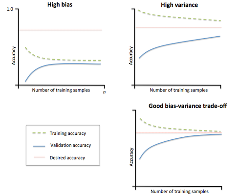
On the learning curve, we vary the train-test split on the x-axis and calculate the accuracy of the model on the training and validation datasets. If the gap between them is too wide, it’s too complex (i.e. over-fitting). If neither one of the curves is hitting the desired accuracy and the gap between the curves is too small, the dataset is highly biased.
ROC
When dealing with fraud datasets with heavy class imbalance, a classification score does not make much sense. Instead, Receiver Operating Characteristic or ROC curves offer a better alternative.

The 45 degree line is the random line, where the Area Under the Curve or AUC is 0.5 . The further the curve from this line, the higher the AUC and better the model. The highest a model can get is an AUC of 1, where the curve forms a right angled triangle. The ROC curve can also help debug a model. For example, if the bottom left corner of the curve is closer to the random line, it implies that the model is misclassifying at Y=0. Whereas, if it is random on the top right, it implies the errors are occurring at Y=1. Also, if there are spikes on the curve (as opposed to being smooth), it implies the model is not stable. When dealing with fraud models, ROC is your best friend.
Additional Materials
Bio: Syed Sadat Nazrul is using Machine Learning to catch cyber and financial criminals by day... and writing cool blogs by night.
Original. Reposted with permission.
Related:
- The Two Sides of Getting a Job as a Data Scientist
- How to Survive Your Data Science Interview
- A Guide to Hiring Data Scientists