Deep learning scaling is predictable, empirically
This study starts with a simple question: “how can we improve the state of the art in deep learning?”
Deep learning scaling is predictable, empirically Hestness et al., arXiv, Dec.2017
With thanks to Nathan Benaich for highlighting this paper in his excellent summary of the AI world in 1Q18
This is a really wonderful study with far-reaching implications that could even impact company strategies in some cases. It starts with a simple question: “how can we improve the state of the art in deep learning?” We have three main lines of attack:
- We can search for improved model architectures.
- We can scale computation.
- We can create larger training data sets.
As DL application domains grow, we would like a deeper understanding of the relationships between training set size, computational scale, and model accuracy improvements to advance the state-of-the-art.
Finding better model architectures often depends on ‘unreliable epiphany,’ and as the results show, has limited impact compared to increasing the amount of data available. We’ve known this for some time of course, including from the 2009 Google paper, ‘The unreasonable effectiveness of data.’ The results from today’s paper help us to quantify the data advantage across a range of deep learning applications. The key to understanding is captured in the following equation:
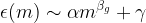
Which says that the generalisation error  as a function of the amount of training data
  , follows a power-law with exponent
  . Empirically,
  usually seems to be in the range -0.07 and -0.35. With error of course, lower is better, hence the negative exponents. We normally plot power-laws on log-log graphs, where they result in straight lines with the gradient indicating the exponent.
Making better models can move the y-intercept down (until we reach the irreducible error level), but doesn’t seem to impact the power law coefficient. On the other hand, more data puts us on an power law path of improvement.

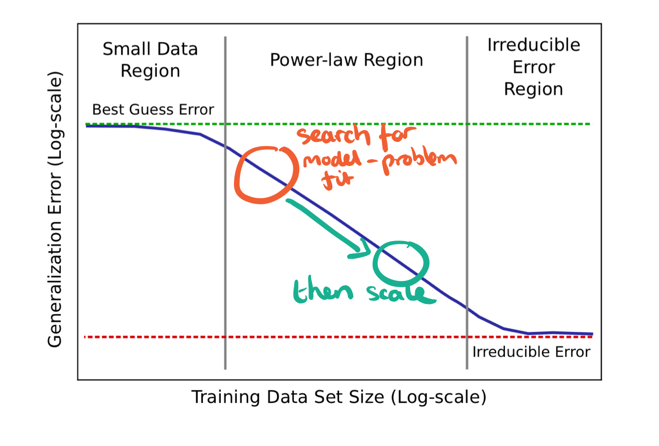
The three learning zones
The learning curves for real applications can be broken down into three regions:

- The small data region is where models struggle to learn from insufficient data and models can only perform as well as ‘best’ or ‘random’ guessing.
- The middle region is the power-law region, where the power-law exponent defines the steepness of the curve (slope on a log-log scale). The exponent is an indicator of the difficulty for models to represent the data generating function.
“Results in this paper indicate that the power-law exponent is unlikely to be easily predicted with prior theory and probably dependent on aspects of the problem domain or data distribution.”
- The irreducible error region is the non-zero lower-bound error past which models will be unable to improve. With sufficiently large training sets, models saturate in this region.
On model size
We expect the number of model parameters to fit a data set should follow
where
 where
where  is the required model size to fin a training set of size
 ![\beta_p \in [0.5,1]](https://s0.wp.com/latex.php?latex=%5Cbeta_p+%5Cin+%5B0.5%2C1%5D&bg=ffffff&fg=000000&s=1) .
.Best-fit models grow sublinearly in training shard size. Higher values of  indicate models that make less effective use of extra parameters on larger data sets. Despite model size scaling differences though, “for a given model architecture, we can accurately predict the model size that will best fit increasingly larger data sets.”
Implications of the power-law
Predictable learning curves and model size scaling indicate some significant implications on how DL could proceed. For machine learning practitioners and researchers, predictable scaling can aid model and optimization debugging and iteration time, and offer a way to estimate the most impactful next steps to improve model accuracy. Operationally, predictable curves can guid decision making about whether or how to grow data sets or computation.
One interesting consequence is that model exploration can be done on smaller data sets (and hence faster / cheaper). The data set needs to be large enough to show accuracy in the power-law region of the curve. Then the most promising models can be scaled to larger data sets to ensure proportional accuracy gains. This works because growing training sets and models is likely to result in the same relative gains across models. When building a company we look for product-market fit before scaling the business. In deep learning it seems the analogy is to look for model-problem fit before scaling, a search then scale strategy:
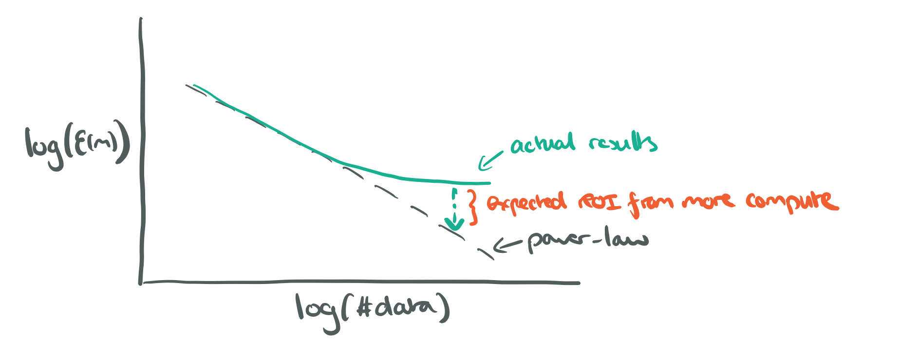
If you need to make a business decision about the return on investment, or likely accuracy improvement, from investing in the collection of more data, the power-law can help you predict returns:

Conversely, if generalisation error within the power-law region drifts from the power-law predictions, it’s a clue that increasing model size might help, or a more extensive hyperparameter search (i.e., more compute), might help:
…predictable learning and model size curves may offer a way to project the compute requirements to reach a particular accuracy level.
Can you beat the power law?
Model architecture improvements (e.g., increasing model depth) seem only to shift learning curves down, but not improve the power-law exponent.
We have yet to find factors that affect the power-law exponent. To beat the power-law as we increase data set size, models would need to learn more concepts with successively less data. In other words, models must successively extract more marginal information from each additional training sample.
If we can find ways to improve the power-law exponent though, then the potential accuracy improvements in some problem domains are ‘immense.’
The empirical data
The empirical data to back all this up was collected by testing various training data sizes (in powers of two) with state-of-the-art deep learning models in a number of different domains.
Here are the neural machine translation learning curves. On the right you can see results for the best-fit model at each training set size. As training set sizes grow, the empirical error tends away from the power-law trend, and a more exhaustive hyperparameter search would be needed to bring it back in line.

The next domain is word language models. A variety of model architectures are used, and although they differ appreciably, they all show the same learning curve profile as characterised by the power-law exponent.

And here are the results for character language models:

With image classification, we see the ‘small data region’ appear on the plots when there is insufficient data to learn a good classifier:

Finally, here’s speech recognition:

We empirically validate that DL model accuracy improves as a power-law as we grow training sets for state-of-the-art (SOTA) model architectures in four machine learning domains: machine translation, language modeling, image processing, and speech recognition. These power-law learning curves exist across all tested domains, model architectures, optimizers, and loss functions.
Original. Reposted with permission.
Related:
- How to Make AI More Accessible
- Are High Level APIs Dumbing Down Machine Learning?
- Derivation of Convolutional Neural Network from Fully Connected Network Step-By-Step