Basic Image Data Analysis Using Numpy and OpenCV – Part 1
Accessing the internal component of digital images using Python packages becomes more convenient to understand its properties as well as nature.
Introduction: A Little Bit About Pixel
Computer store images as a mosaic of tiny squares. This is like the ancient art form of tile mosaic, or the melting bead kits kids play with today. Now, if these square tiles are too big, it’s then hard to make smooth edges and curves. The more and smaller tiles we use, the smoother or as we say less pixelated, image will be. These sometimes gets referred to as resolution of the images.
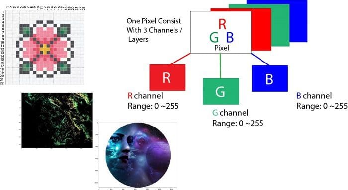
Vector graphics are somewhat different method of storing images that aims to avoid pixel related issues. But even vector images, in the end, are displayed as a mosaic of pixels. The word pixel means a picture element. A simple way to describe each pixel is using a combination of three colors, namely Red, Green, Blue. This is what we call an RGB image.
In an RGB image, each pixel is represented by three 8 bit numbers associated to the values for Red, Green, Blue respectively. Eventually using a magnifying glass, if we zoom a picture, we’ll see the picture is made up of tiny dots of little light or more specifically the pixels and what more interesting is to see that those tiny dots of little light are actually multiple tiny dots of little light of different colors which are nothing but Red, Green, Blue channels.
Pixel together from far away, create an image and upfront they’re just little lights that are ON and OFF. The combination of those create images and basically what we see on screen every single day.
Every photograph, in digital form, is made up of pixels. They are the smallest unit of information that makes up a picture. Usually round or square, they are typically arranged in a 2-dimensional grid.
Now, if all three values are at full intensity, that means they’re 255, it then shows as white and if all three colors are muted, or has the value of 0, the color shows as black. The combination of these three will, in turn, give us a specific shade of the pixel color. Since each number is an 8-bit number, the values range from 0-255.
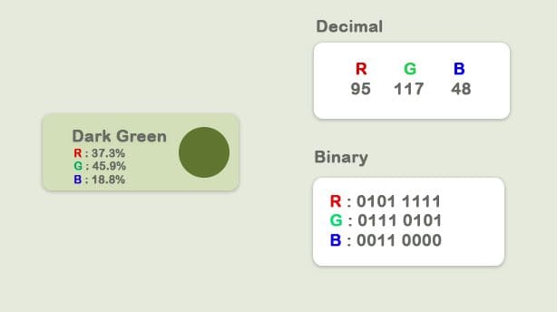
Combination of these three color will possess tends to the highest value among them. Since each value can have 256 different intensity or brightness value, it makes 16.8 million total shades.
Here, we'll observe some following stuffs which is very basic fundamental image data analysis with Numpy and some concern Python packages, like imageio , matplotlib etc.
- Importing images and observe its properties
- Splitting the layers
- Grey scale
- Using Logical Operator on pixel values
- Masking using Logical Operator
- Satellite Image Data Analysis
Importing Image
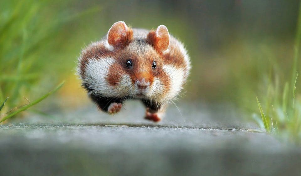
Now let’s load an image and observe its various properties in general.
if__name__=='__main__':
import imageio
import matplotlib.pyplotasplt
%matplotlibinline

pic=imageio.imread('F:/demo_2.jpg')
plt.figure(figsize=(15,15))

plt.imshow(pic)
Observe Basic Properties of Image
print('Type of the image : ',type(pic))
print()
print('Shape of the image : {}'.format(pic.shape))
print('Image Hight {}'.format(pic.shape[0]))
print('Image Width {}'.format(pic.shape[1]))
print('Dimension of Image {}'.format(pic.ndim))

-Output:

Type of the image :<class 'imageio.core.util.Image'>

Shape of the image : (562, 960, 3)
Image Height 562
Image Width 960
Dimension of Image 3
The shape of the ndarray is a three layered matrix. The first two numbers here are length and width, and the third number (i.e. 3) is for the three layers: Red, Green, Blue. So, if we calculate the size of a RGB image, the total size will be counted as height x width x 3
print('Image size {}'.format(pic.size))

print('Maximum RGB value in this image {}'.format(pic.max()))

print('Minimum RGB value in this image {}'.format(pic.min()))

Image size 1618560

Maximum RGB value in this image 255

Minimum RGB value in this image 0
These values are important to verify since the eight-bit color intensity is, cannot be outside of the 0 to 255 range.
Now, using the picture assigned variable we can also access any particular pixel value of an image and further can access each RGB channel separately.
'''

Let's pick a specific pixel located at 100 th Rows and 50 th Column.

And view the RGB value gradually.

'''

pic[100, 50 ]

Image([109, 143,  46], dtype=uint8)
In these case: R = 109; G = 143 ; B = 46 and we can realize that this particular pixel has a lot of GREEN in it. And now we could have also selected one of this number specifically by giving the index value of these three channel. Now we know for this
- 0index value for Red channel
- 1index value for Green channel
- 2index value for Blue channel
But good to know that in OpenCV, Images takes as not RGB but BGR. imageio.imread loads image as RGB (or RGBA), but OpenCV assumes the image to be BGR or BGRA (BGR is the default OpenCV colour format).
# A specific pixel located at Row : 100 ; Column : 50

# Each channel's value of it, gradually R , G , B

print('Value of only R channel {}'.format(pic[ 100, 50, 0]))

print('Value of only G channel {}'.format(pic[ 100, 50, 1]))

print('Value of only B channel {}'.format(pic[ 100, 50, 2]))

Value of only R channel 109

Value of only G channel 143

Value of only B channel 46
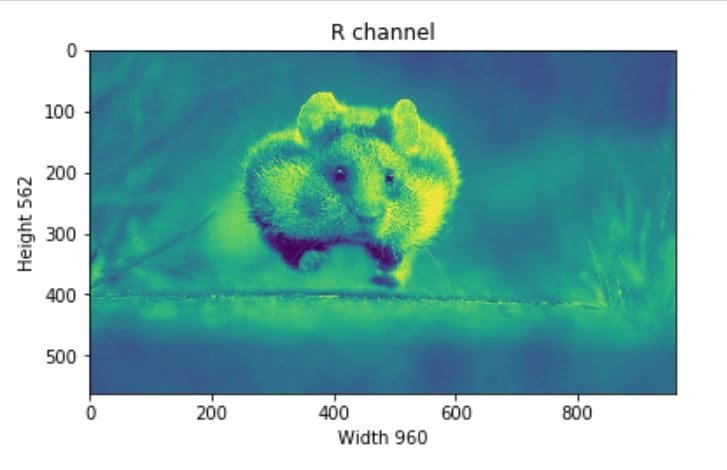
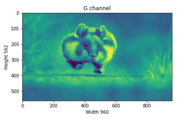
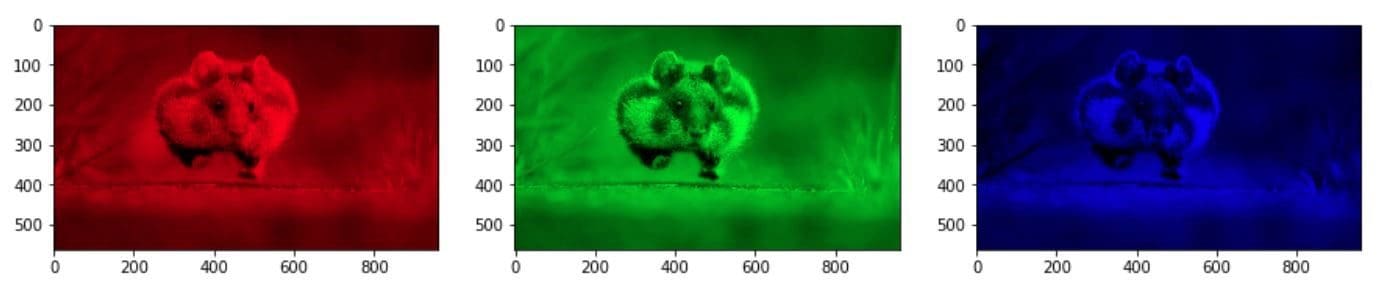
OK, now let’s take a quick view of each channels in the whole image.
plt.title('R channel')

plt.ylabel('Height {}'.format(pic.shape[0]))

plt.xlabel('Width {}'.format(pic.shape[1]))

plt.imshow(pic[ : , : , 0])

plt.show()
plt.title('G channel')

plt.ylabel('Height {}'.format(pic.shape[0]))

plt.xlabel('Width {}'.format(pic.shape[1]))

plt.imshow(pic[ : , : , 1])

plt.show()
plt.title('B channel')

plt.ylabel('Height {}'.format(pic.shape[0]))

plt.xlabel('Width {}'.format(pic.shape[1]))

plt.imshow(pic[ : , : , 2])

plt.show()

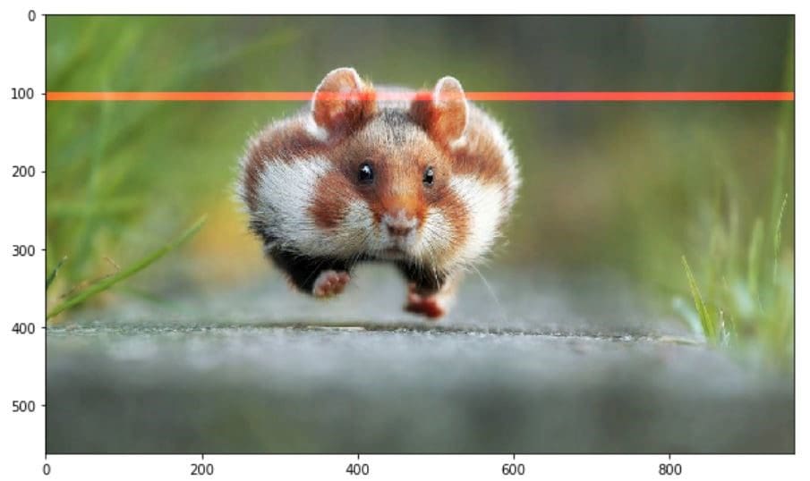
Now, here we can also able to change the number of RGB values. As an example, let’s set the Red, Green, Blue layer for following Rows values to full intensity.
- R channel: Row- 100 to 110
- G channel: Row- 200 to 210
- B channel: Row- 300 to 310
We’ll load the image once, so that we can visualize each change simultaneously
pic =imageio.imread('F:/demo_2.jpg')

pic[50:150 , : , 0] =255# full intensity to those pixel's R channel

plt.figure( figsize= (10,10))

plt.imshow(pic)

plt.show()
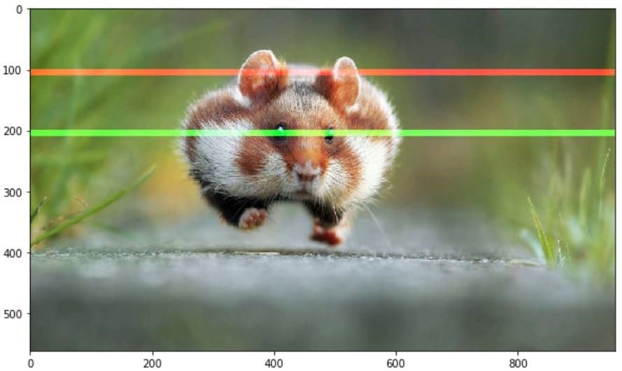
pic[200:300 , : , 1] =255# full intensity to those pixel's G channel

plt.figure( figsize= (10,10))

plt.imshow(pic)

plt.show()
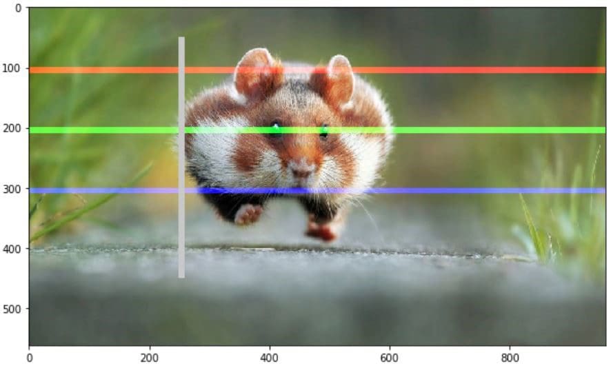
pic[350:450 , : , 2] =255# full intensity to those pixel's B channel

plt.figure( figsize= (10,10))

plt.imshow(pic)

plt.show()

To make it more clear let’s change the column section too and this time we’ll change the RGB channel simultaneously.
# set value 200 of all channels to those pixels which turns them to white

pic[50:450 , 400:600 , [0,1,2] ] =200

plt.figure( figsize= (10,10))

plt.imshow(pic)

plt.show()
Splitting Layers
Now, we know that each pixel of the image is represented by three integers. Splitting the image into separate color components is just a matter of pulling out the correct slice of the image array.
importnumpyasnp

pic=imageio.imread('F:/demo_2.jpg')

fig,ax=plt.subplots(nrows=1,ncols=3,figsize=(15,5))

forc,axinzip(range(3),ax):

# create zero matrix

split_img=np.zeros(pic.shape,dtype="uint8")# 'dtype' by default: 'numpy.float64'

# assing each channel split_img[:,:,c]=pic[:,:,c]

# display each channelax.imshow(split_img)
Greyscale
Black and white images are stored in 2-Dimentional arrays. There’re two types of Black and White images:
- Greyscale: Ranges of shades of grey: 0~ 255
- Binary: Pixel are either black or white: 0or 255
Now, Greyscaling is such process by which an image is converted from a full color to shades of grey. In image processing tools, for example: in OpenCV, many functions uses gray scale images before processing and this is done because it simplifies the image, acting almost as a noise reduction and increasing processing time as there’s less information in the images.
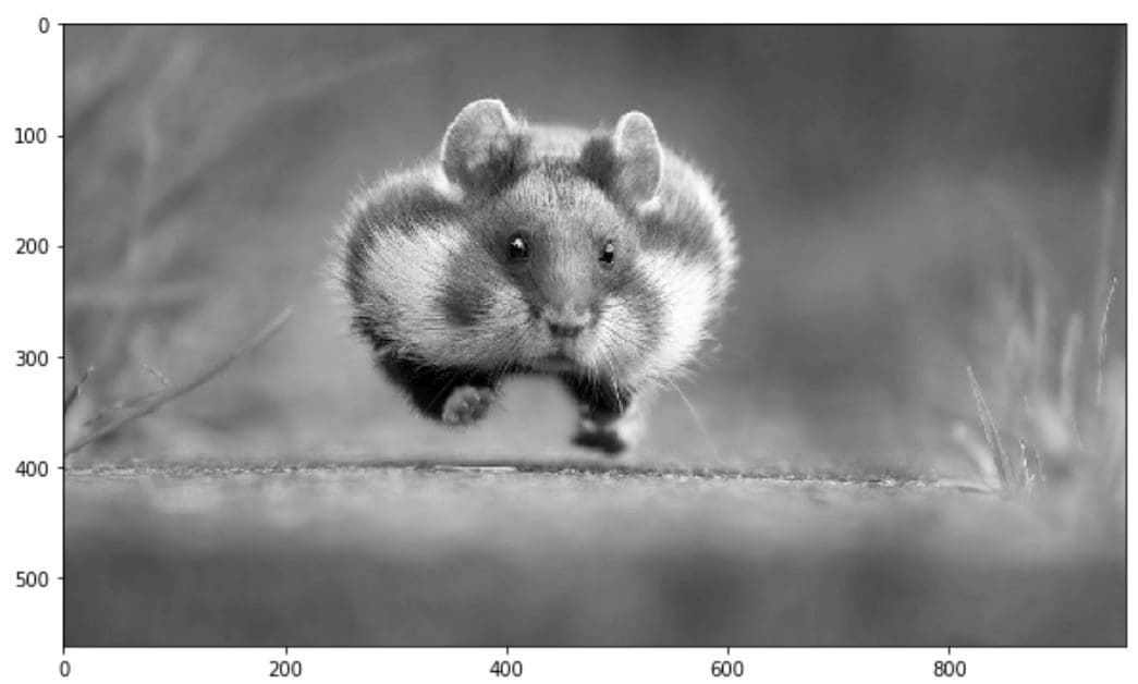
There are a couple of ways to do this in python to convert image to grayscale. But a straight forward way using matplotlib is to take the weighted mean of the RGB value of original image using this formula.
Y' = 0.299 R + 0.587 G + 0.114 B
pic=imageio.imread('F:/demo_2.jpg')
gray=lambdargb:np.dot(rgb[...,:3],[0.299,0.587,0.114])
gray=gray(pic)
plt.figure(figsize=(10,10))
plt.imshow(gray,cmap=plt.get_cmap(name='gray'))
plt.show()
However, the GIMP converting color to grayscale image software has three algorithms to do the task.
Lightness The graylevel will be calculated as
Lightness = ½ × (max(R,G,B) + min(R,G,B))
Luminosity The gray level will be calculated as
Luminosity = 0.21 × R + 0.72 × G + 0.07 × B
Average The gray level will be calculated as
Average Brightness = (R + G + B) ÷ 3
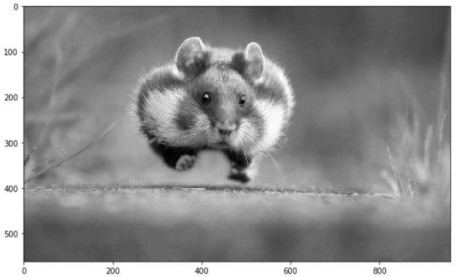
Let’s give a try one of their algorithm, what about Luminosity.
pic=imageio.imread('F:/demo_2.jpg')

gray=lambdargb:np.dot(rgb[...,:3],[0.21,0.72,0.07])

gray=gray(pic)

plt.figure(figsize=(10,10))

plt.imshow(gray,cmap=plt.get_cmap(name='gray'))

plt.show()

'''Let's take a quick overview some the changed properties now the color image.
Like we observe some properties of color image,
same statements are applying now for gray scaled image.'''

print('Type of the image : ',type(gray))

print()

print('Shape of the image : {}'.format(gray.shape))

print('Image Hight {}'.format(gray.shape[0]))

print('Image Width {}'.format(gray.shape[1]))

print('Dimension of Image {}'.format(gray.ndim))

print()

print('Image size {}'.format(gray.size))

print('Maximum RGB value in this image {}'.format(gray.max()))

print('Minimum RGB value in this image {}'.format(gray.min()))

print('Random indexes [X,Y] : {}'.format(gray[100,50]))

Type of the image :<class 'imageio.core.util.Image'>
Shape of the image : (562,960)
Image Height 562
Image Width 960
Dimension of Image 2
Image size 539520
Maximum RGB value in this image 254.9999999997
Minimum RGB value in this image 0.0
Random indexes [X,Y] : 129.07
Type of the image :<class 'imageio.core.util.Image'>
Shape of the image : (562,960)
Image Height 562
Image Width 960
Dimension of Image 2
Image size 539520
Maximum RGB value in this image 254.9999999997
Minimum RGB value in this image 0.0
Random indexes [X,Y] : 129.07
 Type of the image :<class 'imageio.core.util.Image'>
Shape of the image : (562,960)
Image Height 562
Image Width 960
Dimension of Image 2
Image size 539520
Maximum RGB value in this image 254.9999999997
Minimum RGB value in this image 0.0
Random indexes [X,Y] : 129.07
Type of the image :<class 'imageio.core.util.Image'>
Shape of the image : (562,960)
Image Height 562
Image Width 960
Dimension of Image 2
Image size 539520
Maximum RGB value in this image 254.9999999997
Minimum RGB value in this image 0.0
Random indexes [X,Y] : 129.07
Here is the second part.
Bio: Mohammed Innat is currently a fourth year undergraduate student majoring in electronics and communication. He is passionate about applying his knowledge of machine learning and data science to areas in healthcare and crime forecast where better solutions can be engineered in medical sector and security department.
Related:
- DIY Deep Learning Projects
- Unleash a faster Python on Your Data.
- Top 20 Python Libraries for Data Science in 2018