Power Laws in Deep Learning

In pretrained, production quality DNNs, the weight matrices for the Fully Connected (FC ) layers display Fat Tailed Power Law behavior.

comments

By Charles Martin, Machine Learning Specialist

Why Does Deep Learning Work ? If we could get a better handle on this, we could solve some very hard problems in Deep Learning. A new class at Stanford is trying to address this. Here, I review some very new results from my own research (w/UC Berkeley) on the topic which has direct practical application. Here, I will show that

In pretrained, production quality DNNs, the weight matrices for the Fully Connected (FC ) layers display Fat Tailed Power Law behavior.

Setup: the Energy Landscape function

Deep Neural Networks (DNNs) minimize the Energy function defined by their architecture. We define the layer weight matrices $\mathbf{W_{L}}$ , biases, $\mathbf{b_{L}}$ , and activations functions $h_{L}$ , giving

$E_{DNN}=h_{L}(\mathbf{W}_{L}\times h_{L-1}(\mathbf{W}_{L-1}\times h_{L-2}(\cdots)+\mathbf{b}_{L-1})+\mathbf{b}_{L})$

We train the DNN on a labeled data set (d,y), giving the optimization problem

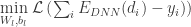
$\underset{W_{l},b_{l}}{\mbox{min}}\;\mathcal{L}\left(\sum_{i}E_{DNN}(d_{i})-y_{i})\right)$

We call this the Energy Landscape because the DNN optimization problem is only parameterized by the weights and biases. Of course, in any real DNN problem, we do have other adjustable parameters, such as the amount of Dropout, the learning rate, the batch size, etc. But these regularization effects simply change the global $E_{DNN}$

The Energy Landscape function changes on each epoch–and do we care about how. In fact, I have argued that $E_{DNN}$ must form an Energy Funnel:

Screen Shot 2018-09-09 at 8.58.26 PM.png

Energy Funnel

But here, for now, we only look at the final result. Once a DNN is trained, what is left are the weights (and biases). We can reuse the weights (and biases) of a pre-trained DNN to build new DNNs with transfer learning. And if we train a bunch of DNNs, we want to know which one is better ?

But, practically, we would really like to identify a very good DNN without peaking at the test data, since every time we peak, and retrain, we risk overtraining our DNN.

I now show we can at least start do this by looking the weights matrices themselves. So let us look at the weights of some pre-trained DNNs.

Pretrained Linear Models in Pytorch

Pytorch comes with several pretrained models, such as AlexNet. To start, we just examine the weight matrices of the Linear / Fully Connected (FC) layers.

pretrained_model = models.alexnet(pretrained=True)
for module in pretrained_model.modules():
     if isinstance(module, nn.Linear):
     ...

The Linear layers have the simplest weight matrices $\mathbf{W}_{l}$ ; they are 2-dimensional tensors, or just rectangular matrices.

Let $\mathbf{W}_{l}$ be an $N\times N$ matrix, where $M\le N$ . We can get the matrix from the pretraing model using:

W = np.array(module.weight.data.clone().cpu())
M, N = np.min(W.shape), np.max(W.shape)

Empirical Spectral Density

How is information concentrated in $\mathbf{W}_{l}$ . For any rectangular matrix, we can form the

Singular Value Decomposition (SVD)

$\mathbf{W}_{l}=\mathbf{U}\mathbf{\Sigma}\mathbf{V}^T$

$\nu_{i}=\Sigma_{ii},\;\;i=1\cdots M$

which is readily computed in scikit learn. We will use the faster TruncatedSVD method, and compute singular values $\nu_{i}$ :

from sklearn.decomposition import TruncatedSVD
svd = TruncatedSVD(n_components=M-1, n_iter=7, random_state=10)
svd.fit(W)
svals = svd.singular_values_

(Technically, we do miss the smallest singular value doing this, but that’s ok. It won’t matter here, and we can always use the pure svd method to be a exact)

Eigenvalues of the Correlation Matrix

We can, alternatively form the eigenvalues of the correlation matrix

$\mathbf{X} = \dfrac{1}{N}\mathbf{W}_{l}^{T}\mathbf{W}_{l}$

$\mathbf{X}\mathbf{v}_{i}=\lambda_{i}\mathbf{v}_{i}$

The eigenvalues are just the square of the singular values.

$\lambda_{i}=\dfrac{1}{N}\nu^{2}_{i}$

Notice here we normalize them by N.

evals = (1/N)*svals*svals

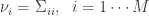
We now form the Empirical Spectral Density (ESD), which is, formally

$\rho_{emp}(\lambda)=\dfrac{1}{N}\sum_{i=1}^{M} \delta\left( \lambda - \lambda_i\right)$

This notation just means compute a histogram of the eigenvalues

import matplotlib.pyplot as plt
plt.hist(evals, bins=100, density=True)

We could also compute the spectral density using a Kernel Density Estimator (KDE); we save this for a future post.

We now look at the ESD of

Pretrained AlexNet

Here, we examine just FC3, the last Linear layer, connecting the model to the labels. The other linear layers, FC1 and FC2, look similar. Below is a histogram for ESD. Notice it is very sharply peaked and has long tail, extending out past 40.

We can get a better view of the heavy tailed behavior by zooming in.

The red curve is a fit of the ESD to the Marchenko Pastur (MP) Random Matrix Theory (RMT) result — it is not a very good fit. This means ESD does not resemble Gaussian Random matrix. Instead, it is looks heavy tailed. Which leads to the question…

Do we have a Power Law ?

(Yes do, as we shall see…)

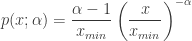
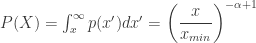
Physicists love to claim they have discovered data that follows a power law:

$P(\lambda)\sim\dfrac{1}{\lambda^{\alpha}},\;\;\alpha>0$

But this is harder to do than it seems. And statisticians love to point this out. Don’t be fooled–we physicists knew this; Sornette’s book has a whole chapter on it. Still, we have to use best practices.

Log Log Histograms

The first thing to do: plot the data on a log-log histogram, and check that this plot is linear–at least in some region. Let’s look at our ESD for AlexNet FC3:

AlexNet FC3: Log log histogram of the Empirical Spectral Density (ESD). Notice the central region is mostly linear, suggesting a power law.

Yes, it is linear–in the central region, for eigenvalue frequencies between roughly ~1 and ~100–and that is most of the distribution.

Why is not linear everywhere? Because it is finite size–there are min and max cutoffs. In the infinite limit, a powerlaw $p(x)$ diverges at $x=0$ , and the tail extends indefinitely as $x\rightarrow\infty$ . In any finite size data set, there will be an $x_{min}$ and $x_{max}$ .

Power Law Fits

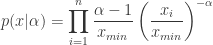
Second, fit the data to a power law, with $x_{min}$ and $x_{max}$ in mind. The most widely available and accepted method the Maximum Likelihood Estimator (MLE), develop by Clauset et. al., and available in the python powerlaw package.

import powerlaw
fit = powerlaw.Fit(evals, xmax=np.max(evals))
alpha, D = fit.alpha, fit.D

The D value is a quality metric, the KS distance. There are other options as well. The smaller D, the better. The table below shows typical values of good fits.

Linear Log Log Plots

The powerlaw package also makes some great plots. Below is a log log plot generated for our fit of FC3, for the central region of the ESD. The filled lines represent our fits, and the dotted lines are actual power lawPDF (blue) and CCDF (red). The filled lines look like straight lines and overlap the dotted lines–so this fit looks pretty good.

AlexNet FC3: Log Log plot of the central region of the Empirical Spectral Density and best Powerlaw fits: pdf (blue) and ccdf (red)

Is this enough ? Not yet…

Quality of the Estimator

We still need to know, do we have enough data to get a good estimate for $\alpha$ , what are our error bars, and what kind of systematic errors might we get?

This so-called statistically valid MLE estimator actually only works properly for $\alpha\in[1.5,3.5]$ .
And we need a lot of data points…more than we have singular values $\nu_{i}$

We can calibrate the estimator by generating some modest size (N=1000) random power law datasets using the numpy Pareto function, where

$\alpha=\mu+1$

and then fitting these with the PowerLaw package. We get the following curve

Powerlaw fits of exponent compared to data generated from a Pareto distribution, N=1000. Notice that the estimator works best for exponents between 1.5 and 3.5

The green line is a perfect estimate. The Powerlaw package overestimates small $\alpha<1.5$ and underestimates large $\alpha>3.5$ . Fortunately, most of our fits lie in the good range.

Is a Power law the best model ?

A good fit is not enough. We also should ensure that no other obvious model is a better fit. The power law package lets us test out fit against other common (long tailed) choices, namely

exponential (EXP)
stretched_exponential (S_EXP)
log normal (LOG_N)
truncated power law (TPL)

For example, to check if our data is better fit by a log normal distribution, we run

R, p = fit.distribution_compare('powerlaw', 'lognormal', normalized_ratio=True)

and R and the the p-value. If if R<0 and p <= 0.05, then we can conclude that a power law is a better model.

Note that sometimes, for $\alpha\leq2$ , the best model may be a truncated power law (TPL). This happens because our data sets are pretty small, and the tails of our ESDs fall off pretty fast. A TPL is just a power law (PL) with an exponentially decaying tail, and it may seem to be a better fit for small data, fixed size sets. Also, the TPL also has 2 parameters, whereas the PL has only 1, so it is not unexpected that the TPL would fit the data better.

More Pretrained Models: Linear Layers

Below we fit the linear layers of the many pretrained models in pytorch. All fit a power law (PL) or truncated power law (TPL)

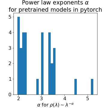
Powerlaw exponents for ESD of Fully Connected / Linear layers of numerous pretrained ImageNet models currently available in pytorch.

The table below lists all the fits, with the Best Fit and the KS statistic D.

Notice that all the power law exponents lie in the range 2-4, except for a couple outliers.

$\alpha\in[2,4]$

This is pretty fortunate since out PL estimator only works well around this range. This is also pretty remarkable because it suggests there is…

Universality in Deep Learning:

There is a deep connection between this range of exponents and some (relatively) recent results in Random Matrix Theory (RMT). Indeed, this seems to suggest that Deep Learning systems display the kind of Universality seen in Self Organized systems, like real spiking neurons. We will examine this in a future post.

Practical Applications:

Training DNNs is hard. There are many tricks one has to use. And you have to monitor the training process carefully.

Here we suggest that the ESDs of the Linear / FC layers of a well trained DNN will display power law behavior. And the exponents will be between 2 and 4.

Counterexample: Inception V3

A counter example is Inception V3. Both FC layers 226 and 302 have unusually large $\alpha$ exponents. Looking closer at Layer 222, the ESDs is not a power law at all, but rather bi-model heavy tailed distribution.

We conjecture that as good as Inception V3 is, perhaps it could be further optimized. It would be interesting to see if anyone can show this.

Appendix:

Derivation of the MLE PowerLaw estimator
The commonly accepted method uses Maximum Likelihood Estimator (MLE). This

$p(x;\alpha)\sim x^{-\alpha}$
$p(x;\alpha)=\dfrac{\alpha-1}{x_{min}}\left(\dfrac{x}{x_{min}}\right)^{-\alpha}$
$P(X)=\int_{x}^{\infty}p(x')dx'=\left(\dfrac{x}{x_{min}}\right)^{-\alpha+1}$

The conditional probability is defined by evaluating $p(x;\alpha)$ on a data set (of size n)

$p(x|\alpha)=\displaystyle\prod_{i=1}^{n}\dfrac{\alpha-1}{x_{min}}\left(\dfrac{x_{i}}{x_{min}}\right)^{-\alpha}$

The log likelihood is

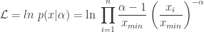
$\mathcal{L}=ln\;p(x|\alpha)=\ln\;\displaystyle\prod_{i=1}^{n}\dfrac{\alpha-1}{x_{min}}\left(\dfrac{x_{i}}{x_{min}}\right)^{-\alpha}$

Which is easily reduced to

$=\displaystyle\sum_{i=1}^{n}\Big[ln(\alpha-1)-ln(x_{min})-\alpha\;ln\left(\dfrac{x_{i}}{x_{min}}\right)\Big]$
$=n\;ln(\alpha-1)-n\; ln(x_{min})-\alpha\; ln\displaystyle\sum_{i=1}^{n}\left(\dfrac{x_{i}}{x_{min}}\right)$

The maximum likelihood occurs when

$\dfrac{\partial\mathcal{L}}{\partial\alpha}=0$

The MLE estimate, for a given $x_{min}$ , is:

$\hat{\alpha}=1+n\Big[\displaystyle\sum_{i=1}^{n}ln\dfrac{x_{i}}{x_{min}}\Big]^{-1}$

We can either input $x_{min}$ , or search for the best possible estimate (as explained in the Clauset et. al. paper).

Notice, however, that this estimator does not explicitly take $x_{max}$ into account. And for this reason it seems to be very limited in its application. A better method, such as developed recently by Thurner (but not yet coded in python), may prove more robust for a larger range of exponents.

Universality in NLP Models:

Similar results arise in the Linear and Attention layers in NLP models. Below we see the power law fits for 85 Linear layers in the 6 pretrained models from AllenNLP

Screen Shot 2018-09-13 at 12.37.26 PM

80% of the linear layers have $\alpha\in[2,4]$

Extending this to Convolutional (Conv2D) Layers:

We can naively extend these results to Conv2D layers by reshaping the Conv2D 4-D Tensors back into rectangular 2D matrices. Doing this, and repeating the fits, we see very different results:

Many Conv2D layers show very high exponents. What could this mean?

The PL estimator is terrible for large exponents. We need to implement a more reliable PL estimator before we can start looking at Conv2D layers.
We reshaped the Conv2D layers in a naive way. Perhaps there is some more clever way to reshare the Conv2D Tensors into 2D arrays that better reflects the underlying math
Or, perhaps it is simply that the Linear layers, being fully connected, are also fully correlated, whereas the Conv2D layers do less work.

It will be very exciting to find out.

Jupyter Notebooks

Code for this study, and future work, is available in this repo.

Video Presentations

Research talks are available on my youtube channel. Please Subscribe

Bio: Dr. Charles Martin is a specialist in Machine Learning, Data Science, Deep Learning, and Artificial Intelligence. He helped develop Aardvark, a Machine Learning / NLP startup acquired by Google in 2010. He currently runs a boutique consulting firm specializing in software development, machine learning and AI. His clients include Wall Street firms, Big Pharma, Telecom, eCommerce, early and late stage startups, and the largest Internet companies such as eHow, eBay, GoDaddy, etc.

Original. Reposted with permission.

Related:

Power Laws in Deep Learning

Setup: the Energy Landscape function

Empirical Spectral Density

Do we have a Power Law ?

Appendix:

More On This Topic

Latest Posts

Top Posts