Multi-Class Text Classification Model Comparison and Selection
This is what we are going to do today: use everything that we have presented about text classification in the previous articles (and more) and comparing between the text classification models we trained in order to choose the most accurate one for our problem.
By Susan Li, Sr. Data Scientist

Photo credit: Pixabay
When working on a supervised machine learning problem with a given data set, we try different algorithms and techniques to search for models to produce general hypotheses, which then make the most accurate predictions possible about future instances. The same principles apply to text (or document) classification where there are many models can be used to train a text classifier. The answer to the question “What machine learning model should I use?” is always “It depends.” Even the most experienced data scientists can’t tell which algorithm will perform best before experimenting them.
This is what we are going to do today: use everything that we have presented about text classification in the previous articles (and more) and comparing between the text classification models we trained in order to choose the most accurate one for our problem.
The Data
We are using a relatively large data set of Stack Overflow questions and tags. The data is available in Google BigQuery, it is also publicly available at this Cloud Storage URL: https://storage.googleapis.com/tensorflow-workshop-examples/stack-overflow-data.csv.
Exploring the Data
10276752
We have over 10 million words in the data.
my_tags = ['java','html','asp.net','c#','ruby-on-rails','jquery','mysql','php','ios','javascript','python','c','css','android','iphone','sql','objective-c','c++','angularjs','.net']
plt.figure(figsize=(10,4))
df.tags.value_counts().plot(kind='bar');
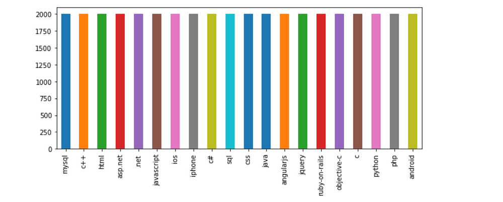
The classes are very well balanced.
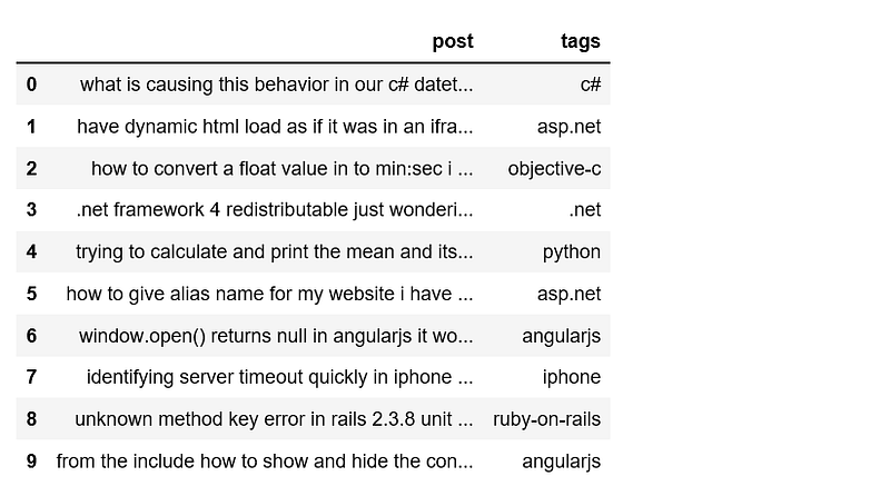
We want to have a look a few post and tag pairs.
def print_plot(index):
    example = df[df.index == index][['post', 'tags']].values[0]
    if len(example) > 0:
        print(example[0])
        print('Tag:', example[1])

print_plot(10)
print_plot(30)

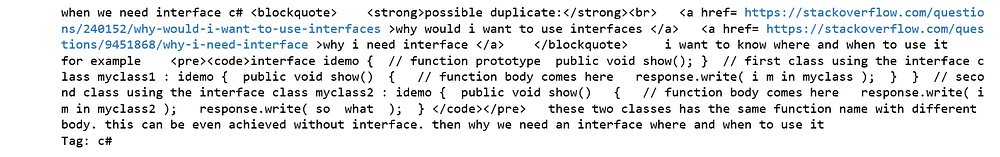
As you can see, the texts need to be cleaned up.
Text Pre-processing
The text cleaning techniques we have seen so far work very well in practice. Depending on the kind of texts you may encounter, it may be relevant to include more complex text cleaning steps. But keep in mind that the more steps we add, the longer the text cleaning will take.
For this particular data set, our text cleaning step includes HTML decoding, remove stop words, change text to lower case, remove punctuation, remove bad characters, and so on.
Now we can have a look a cleaned post:

Way better!
df['post'].apply(lambda x: len(x.split(' '))).sum()
3421180
After text cleaning and removing stop words, we have only over 3 million words to work with!
After splitting the data set, the next steps includes feature engineering. We will convert our text documents to a matrix of token counts (CountVectorizer), then transform a count matrix to a normalized tf-idf representation (tf-idf transformer). After that, we train several classifiers from Scikit-Learn library.
X = df.post
y = df.tags
X_train, X_test, y_train, y_test = train_test_split(X, y, test_size=0.3, random_state = 42)
Naive Bayes Classifier for Multinomial Models
After we have our features, we can train a classifier to try to predict the tag of a post. We will start with a Naive Bayes classifier, which provides a nice baseline for this task. scikit-learn includes several variants of this classifier; the one most suitable for text is the multinomial variant.
To make the vectorizer => transformer => classifier easier to work with, we will use Pipeline class in Scilkit-Learn that behaves like a compound classifier.
We achieved 74% accuracy.
Linear Support Vector Machine
Linear Support Vector Machine is widely regarded as one of the best text classification algorithms.
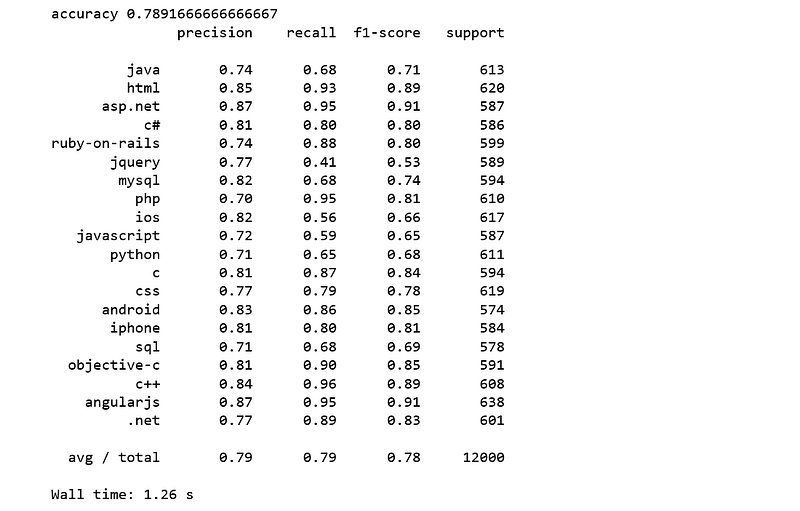
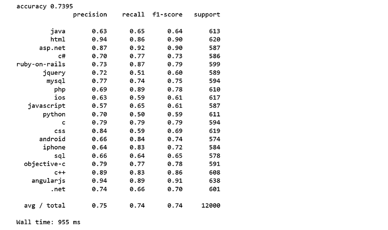
We achieve a higher accuracy score of 79% which is 5% improvement over Naive Bayes.
Logistic Regression
Logistic regression is a simple and easy to understand classification algorithm, and Logistic regression can be easily generalized to multiple classes.
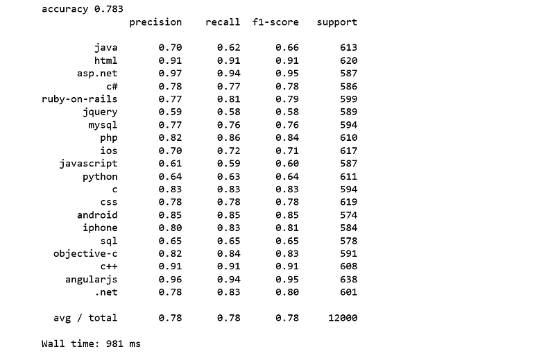
We achieve an accuracy score of 78% which is 4% higher than Naive Bayes and 1% lower than SVM.
As you can see, following some very basic steps and using a simple linear model, we were able to reach as high as an 79% accuracy on this multi-class text classification data set.
Using the same data set, we are going to try some advanced techniques such as word embedding and neural networks.
Now, let’s try some complex features than just simply counting words.