Image by freepik 

Simple linear regression is one of the oldest types of predictive modeling. In a simple linear regression, we have a single feature () and a single continuous target variable (). The goal is to find a mathematical function that describes the relationship between X and y. The simplest form is to try a linear (degree = 1) relationship in the form where and a1 are coefficients to be determined. A quadratic model (degree = 2) takes the form , where , and are regression coefficients to be determined.

Suppose we have a dataset provided in the figure below.

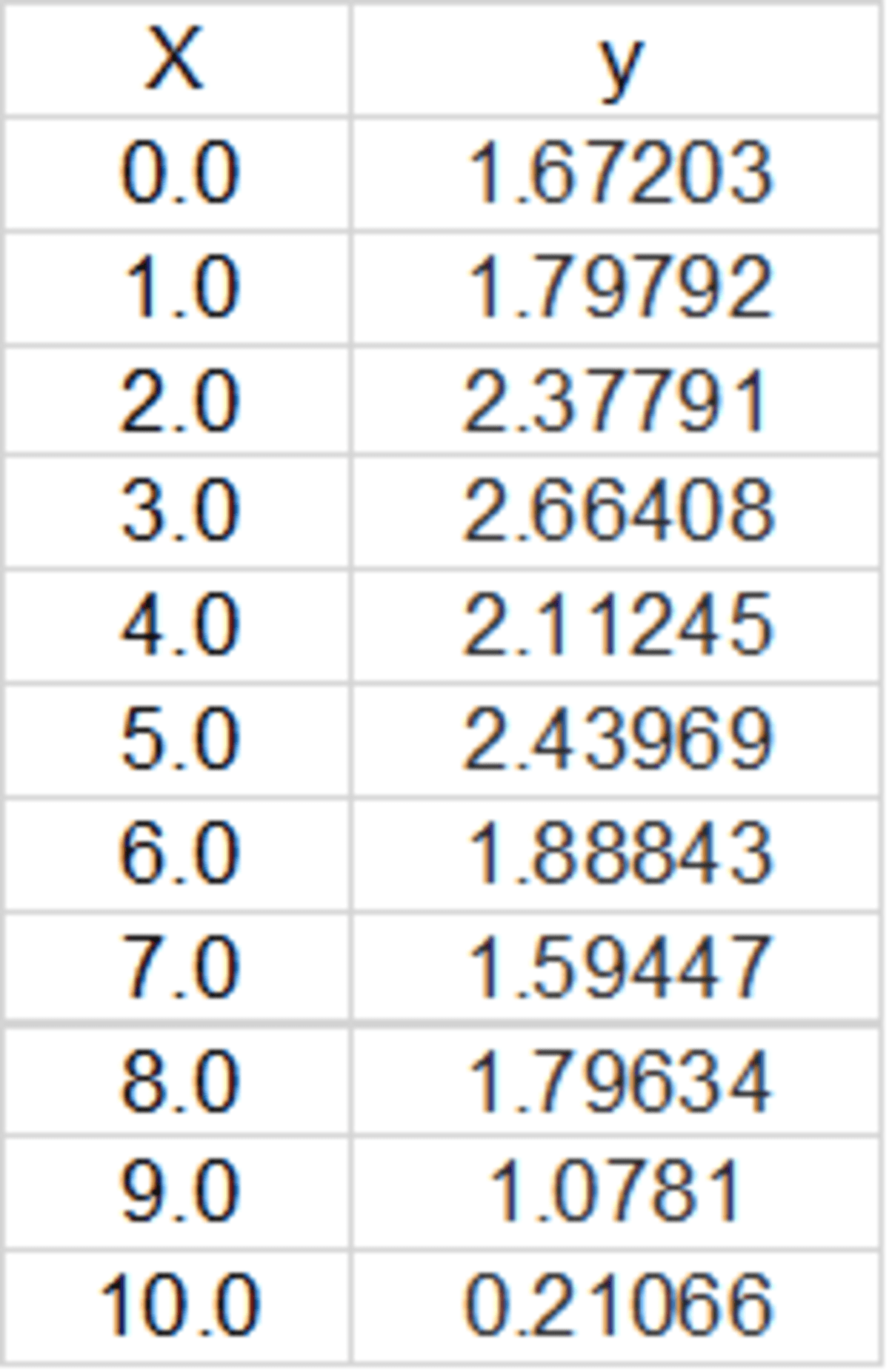
Image by Author

Our goal is to perform regression analysis to quantify the relationship between X and y, that is y = f(X). Once this is obtained, we can then predict a new value for y for any given value for X.

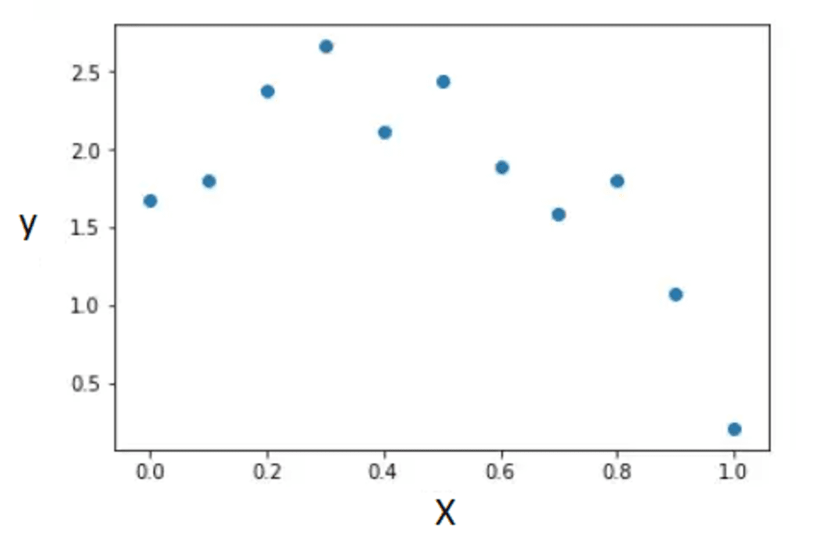
First, we generate a scatter plot to display the relationship between X and y.

import pandas as pd
import pylab
import matplotlib.pyplot as plt
import numpy as np

data = pd.read_csv("file.csv")
X = data.X.values
y = data.y.values

plt.scatter(X, y)
plt.xlabel('X')
plt.ylabel('y')
plt.show()

To perform a polynomial fit of degree =1 for the data, we can use the code below:

degree = 1
model=pylab.polyfit(X,y,degree)
y_pred=pylab.polyval(model,X)
#calculating R-squared value
R2 = 1 - ((y-y_pred)**2).sum()/((y-y.mean())**2).sum()

By changing the degree value to degree = 2, and degree = 10, we can perform higher order polynomial fits to the data. 

The figure below shows a plot of the original and predicted values obtained for different polynomial fits of the data.

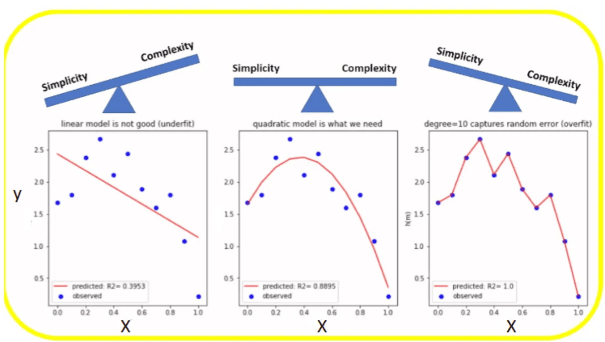
Image by Author

A summary of the goodness of fit score (R2 score) for the different models is given in the table below:

From the figure above, we observe the following:

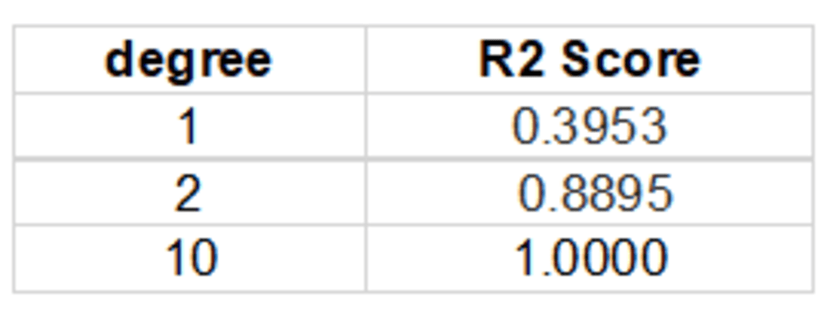
• The linear model (degree = 1) is too simple, and hence underfits the data, leading to a high bias error.
• The higher polynomial model (degree = 10) is too complex, and hence overfits the data, leading to a high variance error.
• The quadratic model (degree = 2) seems to provide the right balance between simplicity and complexity.

Conclusion

In summary, we’ve shown how to perform simple linear regression using python. Generally, a polynomial of any degree could be used to fit the data. However, when selecting the final model, it is important to find the right balance between simplicity and complexity. A model that is too simple underfits the data, leading to high bias error. Likewise, a model that is too complex overfits the data, leading to high variance error. The model with the right balance of simplicity and complexity should be chosen as this model will produce a lower error when applied to new data.
 
 
Benjamin O. Tayo is a Physicist, Data Science Educator, and Writer, as well as the Owner of DataScienceHub. Previously, Benjamin was teaching Engineering and Physics at U. of Central Oklahoma, Grand Canyon U., and Pittsburgh State U.