Four Techniques for Outlier Detection

By Maarit Widmann, Moritz Heine, Rosaria Silipo, Data Scientists at KNIME

Anomalies, or outliers, can be a serious issue when training machine learning algorithms or applying statistical techniques. They are often the result of errors in measurements or exceptional system conditions and therefore do not describe the common functioning of the underlying system. Indeed, the best practice is to implement an outlier removal phase before proceeding with further analysis.

But hold on there! In some cases, outliers can give us information about localized anomalies in the whole system; so the detection of outliers is a valuable process because of the additional information they can provide about your dataset.

There are many techniques to detect and optionally remove outliers from a dataset. In this blog post, we show an implementation in KNIME Analytics Platform of four of the most frequently used - traditional and novel - techniques for outlier detection.

The Dataset and the Outlier Detection Problem

 
The dataset we used to test and compare the proposed outlier detection techniques is the well known airline dataset. The dataset includes information about US domestic flights between 2007 and 2012, such as departure time, arrival time, origin airport, destination airport, time on air, delay at departure, delay on arrival, flight number, vessel number, carrier, and more. Some of those columns could contain anomalies, i.e. outliers.

From the original dataset we extracted a random sample of 1500 flights departing from Chicago O’Hare airport (ORD) in 2007 and 2008.

In order to show how the selected outlier detection techniques work, we focused on finding outliers in terms of average arrival delays at airports, calculated on all flights landing at a given airport. We are looking for those airports that show unusual average arrival delay times.

Four Outlier Detection Techniques

 
Numeric Outlier

This is the simplest, nonparametric outlier detection method in a one dimensional feature space. Here outliers are calculated by means of the IQR (InterQuartile Range).

The first and the third quartile (Q1, Q3) are calculated. An outlier is then a data point x_i that lies outside the interquartile range. That is:

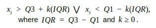
Using the interquartile multiplier value k=1.5, the range limits are the typical upper and lower whiskers of a box plot.

This technique was implemented using the Numeric Outliers node in a workflow built in  KNIME Analytics Platform (Figure 1).

 
Z-Score

 
Z-score is a parametric outlier detection method in a one or low dimensional feature space.

This technique assumes a Gaussian distribution of the data. The outliers are the data points that are in the tails of the distribution and therefore far from the mean. How far depends on a set threshold z_thr for the normalized data points z_i calculated with the formula:

where x_i is a data point, μ is the mean of all x_i and is the standard deviation of all x_i.

An outlier is then a normalized data point which has an absolute value greater than z_thr. That is:

Commonly used z_thr values are 2.5, 3.0 and 3.5.

This technique was implemented using the Row Filter node in a KNIME workflow (Figure 1).

 
DBSCAN

This technique is based on the DBSCAN clustering method. DBSCAN is a non-parametric, density based outlier detection method in a one or multi dimensional feature space.

In the DBSCAN clustering technique, all data points are defined either as Core Points, Border Points or Noise Points.

• Core Points are data points that have at least MinPts neighboring data points within a distance ℇ.
• Border Points are neighbors of a Core Point within the distance ℇ but with less than MinPts neighbors within the distance ℇ.
• All other data points are Noise Points, also identified as outliers.

Outlier detection thus depends on the required number of neighbors MinPts, the distance ℇ and the selected distance measure, like Euclidean or Manhattan.

This technique was implemented using the DBSCAN node in the KNIME workflow in Figure 1.

 
Isolation Forest

This is a non-parametric method for large datasets in a one or multi dimensional feature space.

An important concept in this method is the isolation number.

The isolation number is the number of splits needed to isolate a data point. This number of splits is ascertained by following these steps:

• A point “a” to isolate is selected randomly.
• A random data point “b” is selected that is between the minimum and maximum value and different from “a”.
• If the value of “b” is lower than the value of “a”, the value of “b” becomes the new lower limit.
• If the value of “b” is greater than the value of “a”, the value of “b” becomes the new upper limit.
• This procedure is repeated as long as there are data points other than “a” between the upper and the lower limit.

It requires fewer splits to isolate an outlier than it does to isolate a non-outlier, i.e. an outlier has a lower isolation number in comparison to a non-outlier point. A data point is therefore defined as an outlier if its isolation number is lower than the threshold.

The threshold is defined based on the estimated percentage of outliers in the data, which is the starting point of this outlier detection algorithm.

An explanation with images of the isolation forest technique is available at https://quantdare.com/isolation-forest-algorithm/.

This technique was implemented in the KNIME workflow in Figure 1 by using a few lines of Python code within a Python Script node.

from sklearn.ensemble import IsolationForest
import pandas as pd

clf = IsolationForest(max_samples=100, random_state=42)
table = pd.concat([input_table['Mean(ArrDelay)']], axis=1)
clf.fit(table)
output_table = pd.DataFrame(clf.predict(table))

The Python Script node is part of the KNIME Python Integration, that allows you to write/import Python code into your KNIME workflow.

Implementation in a KNIME Workflow

 
KNIME Analytics Platform is an open source software for data science, covering all your data needs from data ingestion and data blending to data visualization, from machine learning algorithms to data wrangling, from reporting to deployment, and more. It is based on a Graphical User Interface for visual programming, which makes it very intuitive and easy to use, considerably reducing the learning time.

It has been designed to be open to different data formats, data types, data sources, data platforms, as well as external tools, like R and Python for example. It also includes a number of extensions for the analysis of unstructured data, like texts, images, or graphs.

Computing units in KNIME Analytics Platform are small colorful blocks, named “nodes”. Assembling nodes in a pipeline, one after the other, implements a data processing application. A pipeline is called “workflow”.

Given all those characteristics - open source, visual programming, and integration with other data science tools - we have selected it to implement the four techniques for outlier detection described in this post.

The final KNIME workflow implementing these four techniques for outlier detection is reported in Figure 1.The workflow:

1. Reads the data sample inside the Read data metanode.
2. Preprocesses the data and calculate the average arrival delay per airport inside the Preproc metanode.
3. In the next metanode called Density of delay, it normalizes the data and plots the density of the normalized average arrival delays against the density of a standard normal distribution.
4. Detects outliers using the four selected techniques.
5. Visualizes the outlier airports in a map of the US in the MapViz metanode using the KNIME integration with Open Street Maps.

Figure 1: Workflow implementing four outlier detection techniques: Numeric Outlier, Z-score, DBSCAN, Isolation Forest. This workflow is available on the KNIME EXAMPLES server under 02_ETL_Data_Manipulation/01_Filtering/07_Four_Techniques_Outlier_Detection/Four_Techniques_Outlier_Detection.

The Detected Outliers

 
In Figures 2-5 you can see the outlier airports as detected by the different techniques.
The blue circles represent airports with no outlier behavior while the red squares represent airports with outlier behavior. The average arrival delay time defines the size of the markers.

A few airports are consistently identified as outliers by all techniques: Spokane International Airport (GEG), University of Illinois Willard Airport (CMI) and Columbia Metropolitan Airport (CAE). Spokane International Airport (GEG) is the biggest outlier with a very large (180 min) average arrival delay.

A few other airports however are identified by only some of the techniques. For example Louis Armstrong New Orleans International Airport (MSY) has been spotted by only the isolation forest and DBSCAN techniques.

Note that for this particular problem the Z-Score technique identifies the lowest number of outliers, while the DBSCAN technique identifies the highest number of outlier airports.

Only the DBSCAN method (MinPts=3, ℇ=1.5, distance measure Euclidean) and the isolation forest technique (estimated percentage of outliers 10%) find outliers in the early arrival direction.

Figure 2: Outlier airports detected by numeric outlier technique

Figure 3: Outlier airports detected by z-score technique

Figure 4: Outlier airports detected by DBSCAN technique

Figure 5: Outlier airports detected by isolation forest technique

Summary

 
In this blog post, we have described and implemented four different outlier detection techniques in a one dimensional space: the average arrival delay for all US airports between 2007 and 2008 as described in the airline dataset.

The four techniques we investigated are Numeric Outlier, Z-Score, DBSCAN and Isolation Forest methods. Some of them work for one dimensional feature spaces, some for low dimensional spaces, and some extend to high dimensional spaces. Some of the techniques require normalization and a Gaussian distribution of the inspected dimension. Some require a distance measure, and some the calculation of mean and standard deviation.

There are three airports that all the outlier detection techniques identify as outliers. However, only some of the techniques (DBSCAN and Isolation Forest) could identify the outliers in the left tail of the distribution, i.e. those airports where, on average, flights arrived earlier than their scheduled arrival time.

 
References

The theoretical basis for this blog post was taken from:

• Santoyo, Sergio. (2017, September 12). A Brief Overview of Outlier Detection Techniques [Blog post]. https://towardsdatascience.com/a-brief-overview-of-outlier-detection-techniques-1e0b2c19e561

 
Related:

• Removing Outliers Using Standard Deviation in Python
• How to Make Your Machine Learning Models Robust to Outliers
• 8 Common Pitfalls That Can Ruin Your Prediction