 Four Basic Steps in Data Preparation
 Four Basic Steps in Data Preparation
What we would like to do here is introduce four very basic and very general steps in data preparation for machine learning algorithms. We will describe how and why to apply such transformations within a specific example.
By Rosaria Silipo, Head of Data Science Evangelism at KNIME
What are the steps in data preparation? Are there specific steps we need to take for specific problems? The answer is not that straightforward: Practice and knowledge will design the best recipe for each case.
First, there are two types of data preparation: KPI calculation to extract the information from the raw data and data preparation for the data science algorithm. While the first one is domain and business dependent, the second one is more standardized.
In this blog post, we focus on operations to prepare data to feed a machine learning algorithm. There are many of these data operations, some more general and some more dedicated to specific situations. When you consider that there are entire university courses that focus on data preparation operations, the topic is too broad to cover them all in a short article.
What we would like to do here is introduce four very basic and very general steps in data preparation for machine learning algorithms. We will describe how and why to apply such transformations within a specific example.
- Normalization
- Conversion
- Missing value imputation
- Resampling
Our Example: Churn Prediction
Let’s take a simple example in data science: churn prediction. Briefly explained, churn prediction aims at distinguishing between those customers at risk of churning and the other customers. Usually, data from the company’s CRM system are used, including features for customers behavior, demographics, and revenue. Some customers churn, some do not. These data are then used to train a predictive model to distinguish between the two classes of customers.
The problem is a binary classification problem. The output class (churn) has only two possible values: churn “yes” and churn “no”. Any classification algorithm would work here: decision tree, random forest, logistic regression, and so on. Logistic regression is somewhat the historical algorithm, fast to run and easy to interpret. We will adopt it to solve this problem.
Let’s start to build our workflow. First, we read the data from two separate files, a CSV file and an Excel file, then we apply the logistic regression, and finally we write the model to a file.
But hold your horses, Nelly! Let’s have a look at the data first.
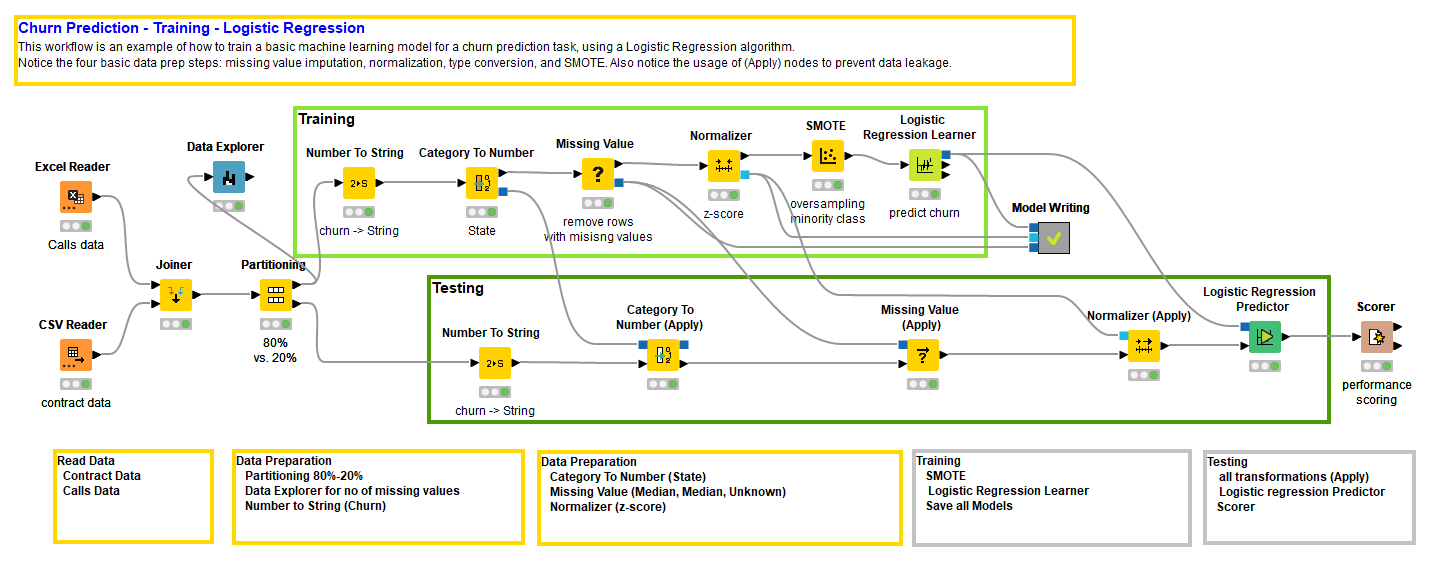
Fig. 1. Workflow to train and evaluate a logistic regression model, including four common data preparation steps (click to enlarge).
Partition the Data to Produce Two Subsets of the Data
Training a model is not enough to claim that we have a good model. We also need to evaluate it by means of an accuracy or an error metric on a separate subset of data. Translated, we need to create a pair of non-overlapping subsets - training set and test set - randomly extracted from the original dataset. For that, we use the Partitioning node. The Partitioning node randomly extracts data from the input data table, in the proportion specified in its configuration window, and produces the two data subsets at the two output ports.
The training set will be used to train the model by the Logistic Regression Learner node and the test set to score the model by the Logistic Regression Predictor node followed by a Scorer node. The Logistic Regression Predictor node generates the churn predictions, and the Scorer node evaluates how correct those predictions are.
Here, we don't include the partitioning operation among the data preparation operations, because it doesn't really change the data. However, this is only our opinion. If you want to include partitioning among the data preparation operations, just change the title from “Four” to “Five basic steps in data preparation” :-)
1. Normalization
Next, logistic regression needs the input data to be normalized into the interval [0, 1], even better if it is Gaussian normalized. Any algorithm including distances or variances will work on normalized data. This is because features with larger ranges affect the calculation of variances and distances and might end up dominating the whole algorithm. Since we want all input features to be considered equally, the normalization of the data is required.
For example, the decision tree relies on probabilities and does not need normalized data, but logistic regression relies on variances and therefore requires previous normalization; many clustering algorithms, like k-Means, rely on distances and therefore require normalization; neural networks use activation functions where the argument falls in [0,1] and therefore also require normalization; and so on. You will learn to recognize which algorithms require normalization and why.
Logistic regression does require Gaussian-normalized data. So, a Normalizer node must be introduced to normalize the training data.
2. Conversion
Logistic Regression works on numerical attributes. This is true for the original algorithm. Sometimes, in some packages, you can see that logistic regression also accepts categorical, i.e. nominal, input features. In this case, a preparation step has been implemented within the logistic regression learning function, to convert the categorical features into numbers. In general, logistic regression works only on numerical features.
Since we want to be in control and not blindly delegate the conversion operation to the logistic regression extended package, we can implement this conversion step on our own. Practically, we want to convert a nominal column into one or more numerical columns. There are two options here:
- Index Encoding. Each nominal value is mapped to a number.
- One hot encoding. Each nominal value creates a new column, whose cells are filled with 1 or 0 depending on the presence or absence of that value in the original column.
The index encoding solution generates one numerical column from one nominal column. However, it introduces an artificial numerical distance between two values due to the mapping function.
The one hot encoding solution does not introduce any artificial distance. However, it generates many columns from the one original column, therefore increasing the dimensionality of the dataset and artificially weighting the original column more.
There is no perfect solution. In the end it is a compromise between accuracy and speed.
In our case, there are two categorical columns in the original dataset: State and Phone. Phone is a unique ID used to identify each customer. We will not use it in our analysis since it does not contain any general information about the customer behavior or contract. State, on the opposite, might contain relevant information. It is plausible that customers from a certain state might be more propense to churn due for example to a local competitor.
To convert the input feature State, we implemented an index-based encoding using the Category to Number node.
On the opposite side of the spectrum, we have the target column Churn, containing the information on whether the customer has churned (1) or not (0). Many classifier training algorithms require a categorical target column for the class labels. In our case, column Churn was read initially as numerical (0/1) and must be converted to the categorical type with a Number To String node.
3. Missing Value Imputation
Another drawback of logistic regression is that it cannot deal with missing values in the data. Some logistic regression learning functions include a missing value strategy. As we said earlier, however, we want to be in control of the whole process. Let’s also decide the strategy for missing value imputation.
There are many strategies in the literature for missing value imputation. You can check the details in the article “Missing Value Imputation: A Review”.
The crudest strategy just ignores the data rows with missing values. It is crude, but if we have data to spare, is not wrong. It becomes problematic when we have little data. In this case, to throw away some data just because some features are missing, might not be the smartest decision.
If we had some knowledge of the domain, we would know what the missing values mean and we would be able to provide a reasonable substitute value.
Since we are clueless and our dataset is really not that big, we need to find some alternative. If we do not want to think, then the adoption of the median, the mean, or the most frequent value is a reasonable choice. If we know nothing, we go with the majority or the middle value. This is the strategy that we have adopted here.
However, if we want to think just a little, we might want to run a little statistic on the dataset, via the Data Explorer node for example, we could estimate how serious the missing value problem is, if at all. As a second step, we could isolate those rows with missing values in the most affected columns. From such observations, an idea might come for a reasonable replacement value. We did that, of course after implementing the missing value strategy in the Missing Value node. And indeed, the view of Data Explorer node showed that our dataset has no missing values. None whatsoever. Oh well! Let’s leave the Missing Value node in there for completion.
4. Resampling
Now the last of the basic questions: are the target classes equally distributed across the dataset?
Well in our case, they are not. There is an imbalance between the two classes of 85% (not churning) vs. 15% (churning). When one class is much less numerous than the other, there is the risk that is going to be overlooked by the training algorithm. If the imbalance is not that strong, then using a stratified sampling strategy for the random extraction of data in the Partitioning node should be enough. However, if the imbalance is stronger, like in this case, it might be useful to perform some resampling before feeding the training algorithm.
To resample, you can either undersample the majority class or oversample the minority class, depending on how much data you are dealing with and if you can afford the luxury of throwing away data from the majority class. This dataset is not that big, so we decided to go for an oversampling of the minority class via the SMOTE algorithm.
Prevent Data Leakage
Now, we have to repeat all these transformations for the test set as well, the same exact transformations as defined in the training branch of the workflow. In order to prevent data leakage, we cannot involve test data in the making of any of those transformations. Therefore, in the test branch of the workflow, we used (Apply) nodes to purely apply the transformations to the test data.
Notice that there is no SMOTE (Apply) node. This is because we either reapply the SMOTE algorithm to oversample the minority class in the test set or we adopt an evaluation metric that takes into account the class imbalance, like the Cohen’s kappa. We chose to evaluate the model quality with the Cohen’s kappa metric.
Packaging and Conclusions
We have reached the end of our workflow (you can download the workflow Four Basic Steps in Data Preparation before Training a Churn Predictor from the KNIME Hub). We have prepared the training data, trained a predictive algorithm on them, prepared the test data using the exact same transformations, applied the trained model on them, and scored the predictions against the real classes. The Scorer node produces a number of accuracy metrics to evaluate the quality of the model. We chose the Cohen’s Kappa, since it measures the algorithm performances on both classes, even if they are highly imbalanced.
We got a Cohen’s Kappa of almost 0.4. Is that the best we can do? We should try to go back, tweak some parameters, and see if we can get a better model. Instead of tweaking the parameters manually, we might even introduce an optimization cycle. Check out the free ebook, From Modeling to Model Evaluation, for more scoring techniques that show a model's performance in a broader context.
We conclude this article now, having introduced four very basic data transformations. We invite you to deepen your knowledge on these four and to investigate other data transformations, such as dimensionality reduction, feature selection, feature engineering, outlier detection, PCA, to name just a few.
Bio: Rosaria Silipo is not only an expert in data mining, machine learning, reporting, and data warehousing, she has become a recognized expert on the KNIME data mining engine, about which she has published three books: KNIME Beginner’s Luck, The KNIME Cookbook, and The KNIME Booklet for SAS Users. Previously Rosaria worked as a freelance data analyst for many companies throughout Europe. She has also led the SAS development group at Viseca (Zürich), implemented the speech-to-text and text-to-speech interfaces in C# at Spoken Translation (Berkeley, California), and developed a number of speech recognition engines in different languages at Nuance Communications (Menlo Park, California). Rosaria gained her doctorate in biomedical engineering in 1996 from the University of Florence, Italy.
As first published on the KNIME Blog.
Original. Reposted with permission.
Related:
- Data Preparation in R using dplyr, with Cheat Sheet!
- Messy Data is Beautiful
- Automated Data Labeling with Machine Learning