Generative Adversarial Networks – Key Milestones and State of the Art
We provide an overview of Generative Adversarial Networks (GANs), discuss challenges in GANs learning, and examine two promising GANs: the RadialGAN, designed for numbers, and the StyleGAN, which does style transfer for images.
By Matt Hergott, MiaBella AI.
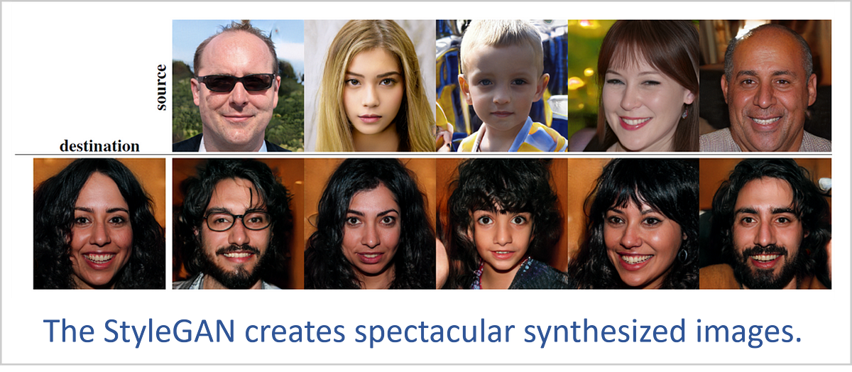
Is December 12, 2018, a day the world changed forever? That Wednesday, a team of researchers at NVIDIA released a dazzling new artificial intelligence design called the StyleGAN.[1] The StyleGAN is a deep learning system based on the idea of a generative adversarial network (GAN), and this model generates ultra-realistic images of people, cars, and households.
Inventions like this could change the way humankind interacts with nearly all media. For instance, when people see images in the news, their first reaction could be to try to determine whether what they are looking at is real or fake.
GANs are some of the more futuristic AI designs, and people have many questions about them: What are GANs? Will I be able to understand them? Can I use GANs for my business analytics, or are they only good at creating images?
This article will try to answer some of these questions. We’ll start with an overview of GANs, then we’ll discuss some challenges in helping GANs to learn. After that, we’ll examine two promising GANs: the RadialGAN,[2]which is designed for numbers, and the StyleGAN, which is focused on images.
The Generative Adversarial Network (GAN)
The original GAN[3] was created by Ian Goodfellow, who described the GAN architecture in a paper published in mid-2014. A GAN consists of two neural networks playing a game with each other. The discriminator tries to determine whether information is real or fake. The other neural network, called a generator, tries to create data that the discriminator thinks is real.
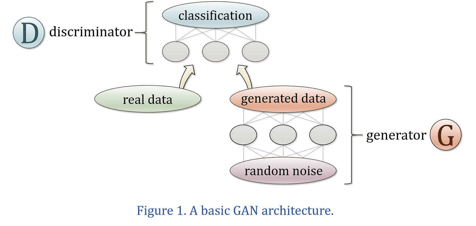
This concept is depicted in Figure 1. The neural network at the top is the discriminator, and its task is to distinguish the training set’s real information from the generator’s creations. In the simplest GAN structure, the generator starts with random data and learns to transform this noise into information that matches the distribution of the real data.
The generator never sees the genuine data; it must learn to create realistic information by receiving feedback from the discriminator. This is called adversarial loss, and when implemented correctly it works surprisingly well. In fact, regularization techniques such as dropout layers are often used in GANs because the generator can overfit the training set through this entirely indirect learning process.
The longer these two neural networks play this game, the more they sharpen each other’s skills. The discriminator becomes very good at detecting fake data while the generator learns to produce information that is indistinguishable from what is observed in the real world.
When we end up with two GAN neural networks that are very good at what they do, how could we use them? A trained discriminator can be used for detecting abnormalities, outliers, and anything out of the ordinary. This could be very valuable in fields such as cybersecurity, radiology, astronomy, and manufacturing.
A skilled generator is used for making creations. Once the generator learns the distribution of the training data, we can sample the generator an unlimited number of times for realistic outputs such as images, language, pharmaceuticals, numerical simulations, and just about anything else one can imagine.
Wasserstein GAN (WGAN)
The original GAN created a lot of excitement when it was first introduced. But there was a problem that showed up immediately: if one of the neural networks started to dominate the other in the GAN game, learning would stop for both. The GAN neural networks are called adversaries, but we want to keep one side from winning so they both can learn for an extended time.
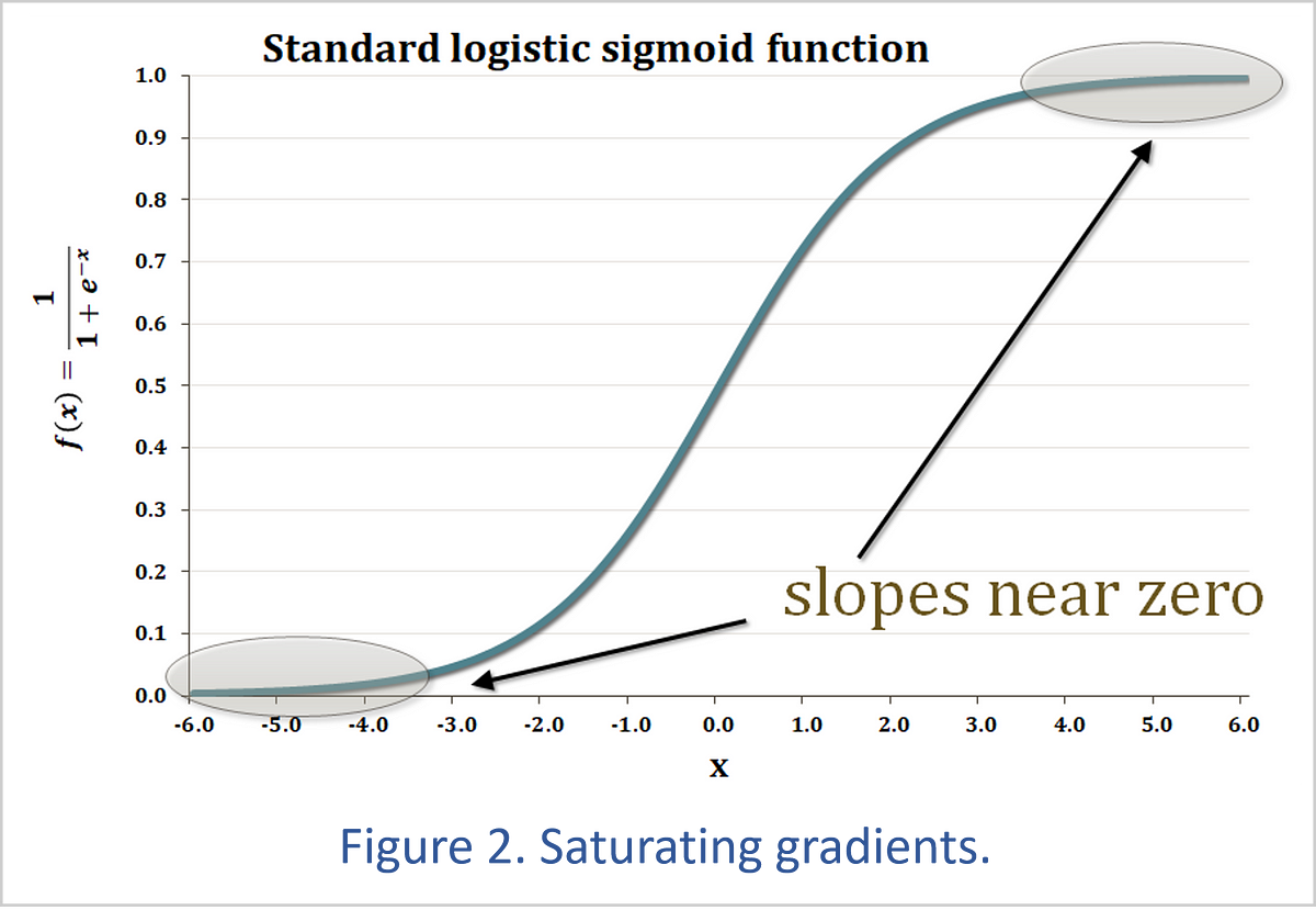
This training dilemma is illustrated in Figure 2. The standard binary classifier is a sigmoid curve — more formally called a standard logistic sigmoid function — that converts an input value into a result between 0 (a negative classification) and 1 (a positive classification). The tail ends of the sigmoid curve are very flat, which means that neural networks can lose their sense of direction if the GAN game ends up far out on one of these tails.
For instance, if the discriminator can always tell that the generator’s creations are fake, the discriminator will always return a 0 to the generator’s training function. If the generator is always able to fool the discriminator, the discriminator always sends a 1 to the generator. In either case, learning stops for both neural networks because neither one is receiving any feedback on how to get better.

An innovation in 2017 made training GANs much more stable. The Wasserstein GAN[4](WGAN) changes the type of response the discriminator sends to the generator. Instead of returning the sigmoid value of the vertical axis, the WGAN returns the input value of the horizontal axis (see Figure 3). In other words, the standard neural network classifier returns f(x), whereas the WGAN returns x.
This means that even if one of the neural networks is always winning, at least the tiny variations that do occur will not get completely flattened out by a sigmoid function. For example, if a GAN discriminator is always able to detect fake data, it might output a value of -100 on one iteration and then -99 on the next iteration. Sending these numbers through a classic sigmoid function makes them indistinguishable at 40+ decimal places. This is why learning stops so easily in the simplest GAN: the generator can end up in a position where it is receiving essentially no direction from the discriminator.
But the WGAN uses the raw numbers (-100 and -99), and this 1% change can be enough to give the generator a path for improvement. This means that learning can continue even if one of the neural networks is overwhelming the other.

The basic WGAN training equations are shown in Figure 4. The terms inside the parentheses represent the desired learning direction of each neural network, and these expressions get multiplied by -1 since we typically optimize in the downhill direction.
If the discriminator is very good at its job, it returns high values for real samples and low values for the fake information coming from the generator. The generator has the opposite goal: it wants the discriminator to assign high values — in other words, false positives — to the generated information.
WGAN Refinements
The Critic
The WGAN authors changed the GAN terminology a bit by referring to the discriminator neural network as a critic. The word discriminator comes from discriminant analysis and reflects a classifier that separates data into categories. The WGAN, on the other hand, returns much richer feedback, and this is somewhat analogous to a written review by a movie critic.
Diverse Results
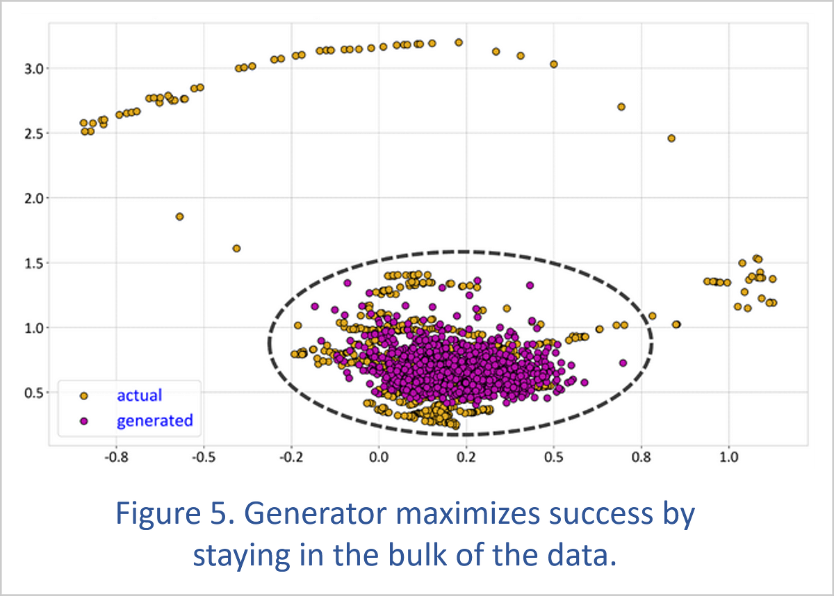
One of the problems people can experience with GANs is that the neural networks appear to be learning properly, but in the end, the generator only re-creates a limited portion of the training distribution. This occurs because the generator can outsmart the training process. If the only instruction the generator receives is to fool the discriminator, the generator can learn to maximize its chance of success by sticking to the most heavily populated portion of the training set.
We typically want a generator to produce a broad range of results, and two common practices help with this.
Minibatch discrimination[5]dynamically collects statistics on a batch of samples — in other words, from multiple observations — at one or more layers of the discriminator neural network. The discriminator then uses these statistics as additional information in its assessment of whether the data set is genuine or fake. If the dispersion of samples is very different between the training set and the generated data, the discriminator can signal to the generator that the generator needs to increase the range of its results.
Another option for producing a wide variety of results is to provide both the generator and the discriminator with extra variables that act as conditioning information to tell the neural networks which environment they are operating in. This is a major advantage when we want to direct a generator to produce creations appropriate for a specific situation.
Optimizers
The WGAN might require some thought as to the best optimizer to use. A sigmoid curve is often called a “squashing” function because it flattens its inputs into a range of 0 to 1.
But the WGAN can return any value at any time, and thus its outputs are nonstationary. For this type of problem, it might be helpful to use optimizers without momentum (like RMSProp[6]) or at least turn down the momentum parameter of an optimizer like adaptive moment estimation (Adam[7]).
WGAN with Gradient Penalty (WGAN-GP)
It turns out that implementing the Wasserstein GAN isn’t quite as simple as eliminating the sigmoid function in the discriminator. The math behind the WGAN requires that the gradients of the discriminator can’t be very steep. In other words, if we alter the inputs to the discriminator neural network, the discriminator’s output can’t change too drastically.
To satisfy this condition, a group of machine learning researchers created the gradient penalty.[8] This technique adds a penalty term to the discriminator’s loss function if the gradients get too sharp, and it pushes the discriminator’s learning process toward flatter gradients.
The general programming pattern for the gradient penalty looks like this:
- Make a randomly weighted combination of the real data and the generator’s manufactured output; this is a way to sample as much of the discriminator’s function range as is feasible.
- Obtain the gradient by measuring how the discriminator’s output changes with respect to this weighted mixture of inputs. This is usually done through a deep learning framework such as TensorFlow’s gradients()function.
- Calculate the norm — in other words, the length — of the gradient and create a penalty based on how far this is from 1.
- Add the result from #3 to the discriminator’s loss function. The discriminator then knows that it needs to learn its job without building a steep relationship between its inputs and output.
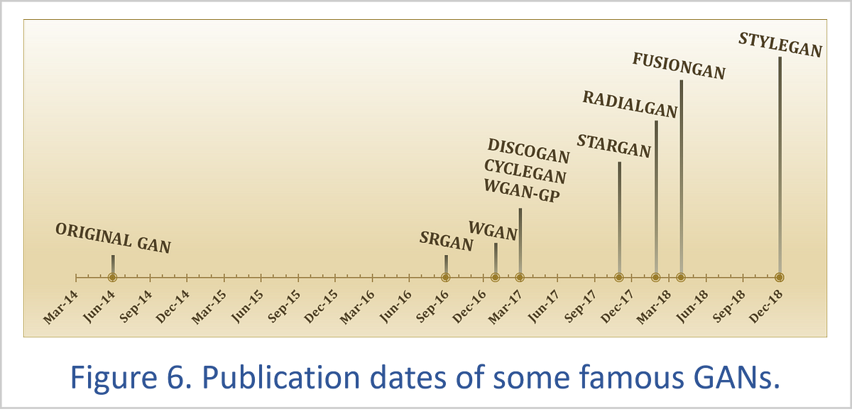
The WGAN-GP approach leads to more stable GAN training and has probably helped to increase the pace of GAN innovation since 2017. For instance, Figure 6 shows how some of the most famous GANs were created over just the past couple of years.
One drawback to the WGAN-GP is its training time. Each iteration requires a calculation of the discriminator’s gradient. Moreover, it is typical to train the discriminator at least 5 times as often as the generator. This is because the excellent feedback a well-trained discriminator gives to the generator should allow the generator to become highly effective with fewer learning iterations.
There is much research being done on how to help GANs learn faster while maintaining the stability of a WGAN-GP.[9]
Sample GANs
Now that we’ve covered the essentials of GANs and how to train them, we’ll look at two very promising GANs. The RadialGAN is designed for numerical analysis, while the StyleGAN received global media coverage for its stunning image creations.
The RadialGAN
Let’s say we are data scientists working for a hospital that wants to evaluate the efficacy of a new medical treatment. Because this procedure is new, our hospital doesn’t have enough data for us to render a credible judgment. We are, however, granted access to other hospitals’ data, and this gives us enough information to give a proper assessment of the new treatment.
But combining data from different hospitals has problems. There is distribution mismatch because the hospitals service very different populations of people. There is also feature mismatch because the hospitals collect their own data sets, use laboratories that give slightly different results, and measure outcomes in varying ways.
This is where the RadialGAN comes in. The RadialGAN first transforms each data set into a latent space, which holds all the data from different sources in a uniform format. The data in the latent space can then be extracted and converted into the feature space of each unique data set.
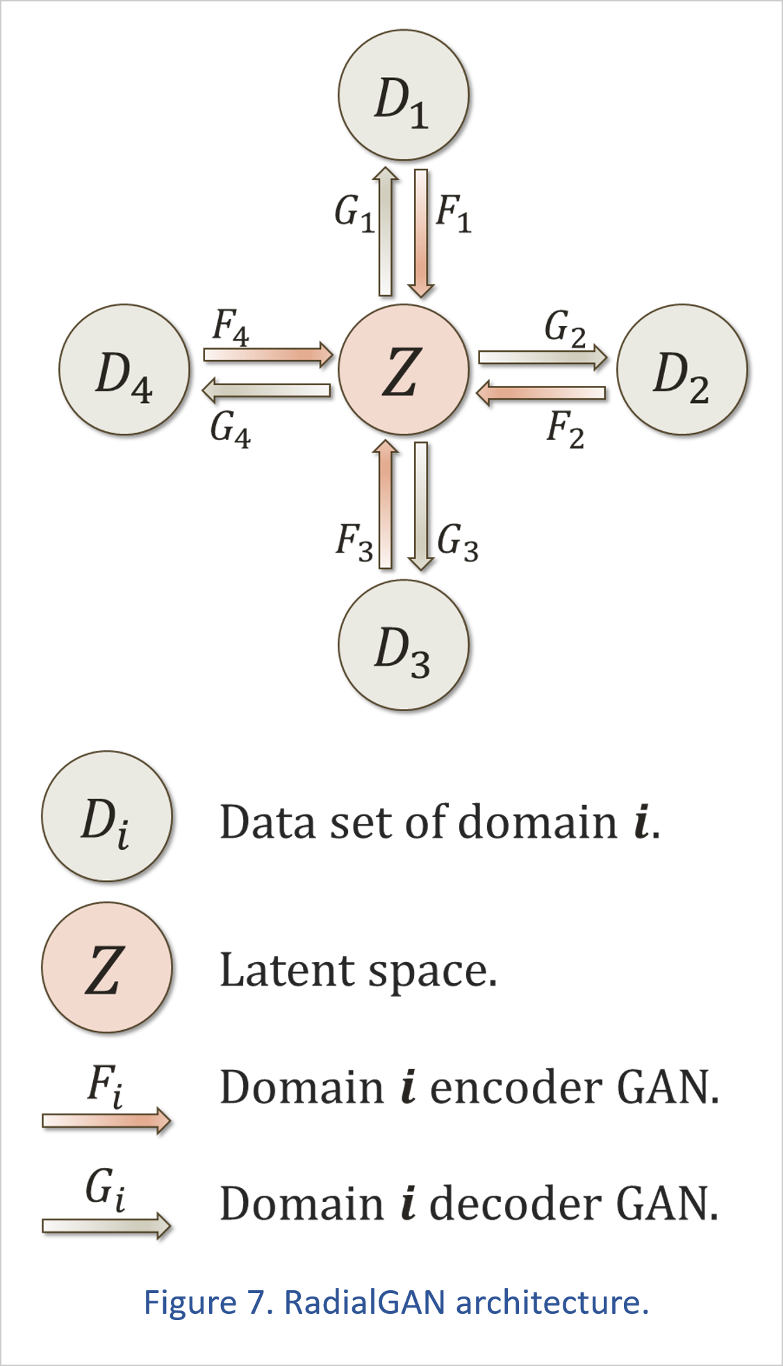
In GAN terminology, these data transformations are referred to as domain transfer, which is when we extract the essential knowledge of a data set and transport that intelligence onto another information set.
In the RadialGAN, each data set has an encoder neural network that transforms the data into the homogeneous structure of the latent space.
Every data source also has a decoder, which is a GAN with a generator that converts information from the latent space into a form consistent with the data set. Each of these decoder GANs has a discriminator that confirms the information coming out of the latent space matches the properties of the target data domain.
This setup makes sure that the domain transfer of information works in both directions and is reversible. This concept is called cycle consistency. It originated with the CycleGAN,[10] and it has become a crucial part of many GAN models.
We train all these neural networks simultaneously, and once the learning process is complete, we can use the RadialGAN to create an augmented data set as shown in Figure 8.

To construct our enhanced data set, we run each of the other data sets through their encoders to transfer that knowledge into the latent space. Then we extract that intelligence from the latent space using our decoder and append the transformed information to our original data set.
The result is a new, larger data set that is bolstered by information from a variety of sources, but which matches the characteristics of the domain we are working in.
The StyleGAN
The spectacular new StyleGAN combines two innovations: the Progressive GAN[11] (ProGAN) and neural style transfer.[12]
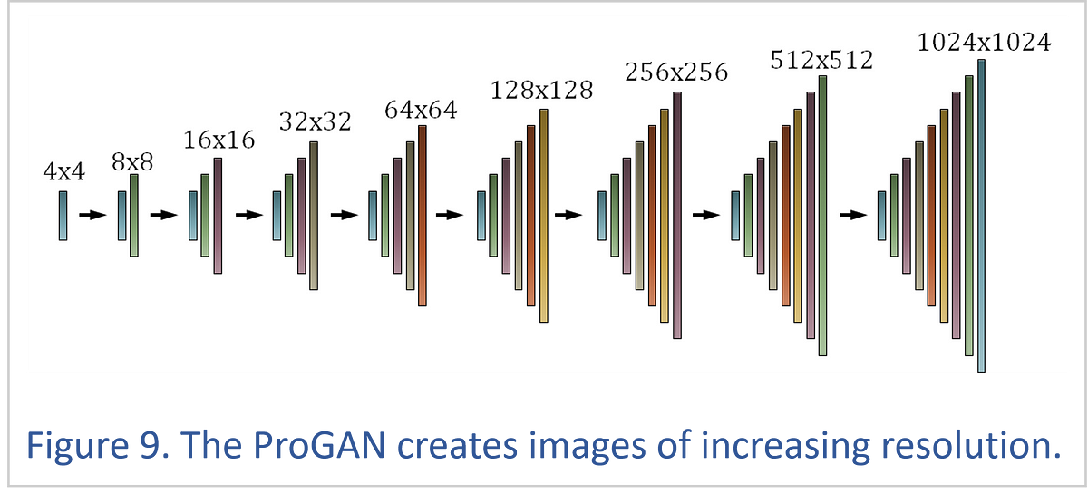
The ProGAN begins by developing a tiny image of 4x4 or 8x8 pixels until this picture is considered realistic by the ProGAN discriminator.
Once this learning is complete, the ProGAN gently adds a higher-resolution layer that also needs to be trained. This process continues until the ProGAN can create 1024x1024-pixel images with amazing realism.

The StyleGAN builds on the ProGAN by bringing in some of the most successful elements of neural style transfer. The original style transfer works by copying the neural network layer correlations of a style image onto a content image. This requires an optimization process that can take too long to be useful in many real-time applications.
Researchers repeatedly made improvements to the classic neural style transfer, and the StyleGAN uses one of the more recent style transfer methods called adaptive instance normalization (AdaIN).[13]
Adaptive instance normalization doesn’t involve an optimization, and it’s therefore a very fast way to transfer styles between images. It’s also very flexible in that it can transfer styles between any images, including those that neural networks have never seen before because they aren’t in any training set.
Applying AdaIN to a convolutional neural network layer of a content image is a simple process:
- Normalize the layer by subtracting its mean and dividing by its standard deviation.
- Scale this normalized layer to match the standard deviation of the style layer.
- Shift the layer by adding in the average value of the style layer.

This sounds more complicated than it really is. All we’re doing is changing the mean and variance of an image’s neural network layers to match the mean and variance of a style image (i.e., the image whose style we want to emulate).
Further refinements to the StyleGAN and AdaIN could include methods like histogram matching, which would transfer more style detail but would also be very fast to calculate.
The StyleGAN is a somewhat complex architecture that incorporates many neural network tools and tricks that have been developed over the past several years. But at its core, the StyleGAN combines the highly effective ProGAN with the successes of neural style transfer to create images that are so realistic they could fundamentally change the relationship people have with the news and entertainment media.
Conclusion
The StyleGAN is a striking example of how generative adversarial networks could transform the way much of the media produces its content and alter how consumers interpret the information they see and hear. The RadialGAN, on the other hand, shows how the features and advantages of GANs can be used to bolster numerical data analysis.
These are two examples of a thriving community of hundreds of innovative GANs that can be used for just about any purpose one can imagine.
Some of the results we’re seeing from GANs look like they come from a different century, and one thing is certain: pioneering AI techniques like GANs are rapidly changing our relationship to technology, and to each other.
References
[1] Tero Karras, Samuli Laine, and Timo Aila
A Style-Based Generator Architecture for Generative Adversarial Networks
[2] Jinsung Yoon, James Jordon, and Mihaela van der Schaar
RadialGAN: Leveraging multiple datasets to improve target-specific predictive models using Generative Adversarial Networks
[3] Ian J. Goodfellow, Jean Pouget-Abadie, Mehdi Mirza, Bing Xu, David Warde-Farley, Sherjil Ozair, Aaron Courville, and Yoshua Bengio
Generative Adversarial Networks
[4] Martin Arjovsky, Soumith Chintala, and Léon Bottou
Wasserstein GAN
[5] Tim Salimans, Ian Goodfellow, Wojciech Zaremba, Vicki Cheung, Alec Radford, and Xi Chen
Improved Techniques for Training GANs
[6] Geoffrey Hinton
Neural Networks for Machine Learning, slide #27: “rprop: Using only the sign of the gradient”
www.cs.toronto.edu/%7Etijmen/csc321/slides/lecture_slides_lec6.pdf
[7] Diederik P. Kingma and Jimmy Ba
Adam: A Method for Stochastic Optimization
[8] Ishaan Gulrajani, Faruk Ahmed, Martin Arjovsky, Vincent Dumoulin, and Aaron Courville
Improved Training of Wasserstein GANs
[9] Lars Mescheder, Andreas Geiger, and Sebastian Nowozin
Which Training Methods for GANs do Actually Converge?
[10] Jun-Yan Zhu, Taesung Park, Phillip Isola, and Alexei A. Efros
Unpaired Image-to-Image Translation using Cycle-Consistent Adversarial Networks
[11] Tero Karras, Timo Aila, Samuli Laine, and Jaakko Lehtinen
Progressive Growing of GANs for Improved Quality, Stability, and Variation
[12] Leon A. Gatys, Alexander S. Ecker, and Matthias Bethge
A Neural Algorithm of Artistic Style
[13] Xun Huang and Serge Belongie
Arbitrary Style Transfer in Real-time with Adaptive Instance Normalization
Original. Reposted with permission.
Bio: Matt Hergott is a Quantitative Researcher at MiaBella AI.
Resources:
- On-line and web-based: Analytics, Data Mining, Data Science, Machine Learning education
- Software for Analytics, Data Science, Data Mining, and Machine Learning
Related: