Graduating in GANs: Going From Understanding Generative Adversarial Networks to Running Your Own

comments

Inception Score

 
Invented in Salimans et al. 2016 in ‘Improved Techniques for Training GANs’, the Inception Score is based on a heuristic that realistic samples should be able to be classified when passed through a pre-trained network, such as Inception on ImageNet. Technically, this means that the sample should have a low entropy softmax prediction vector.

Besides high predictability (low entropy), the Inception Score also evaluates a GAN based on how diverse the generated samples are (e.g. high variance or entropy over the distribution of generated samples). This means that there should not be any dominating classes.

If both these traits are satisfied, there should be a large Inception Score. The way that you combine the two criteria is by evaluating the Kullback-Leibler (KL) divergence between the conditional label distribution of samples and the marginal distribution from all the samples.

Fréchet Inception Distance

 
Introduced by Heusel et al. 2017, FID estimates realism by measuring the distance between the generated distribution of images and the true distribution. FID embeds a set of generated samples into a feature space given by a specific layer of Inception Net. This embedding layer is viewed as as a continuous multivariate Gaussian, then the mean and covariance are estimated for both the generated data and the real data. The Fréchet distance between these two Gaussians (a.k.a Wasserstein-2 distance) is then used to quantify the quality of generated samples. A lower FID corresponds to more similar real and generated samples.

An important note is that FID needs a decent sample size to give good results (suggested size = 50k samples ). If you use too few samples, you will end up over-estimating your actual FID and the estimates will have a large variance.

For a comparison of how Inception Scores and FID scores have differed across papers, see Neal Jean’s post here.

Want to see more?

 
Aji Borji’s paper, ‘Pros and Cons of GAN Evaluation Measures’ includes an excellent table with more exhaustive coverage of GAN evaluation metrics:

Interestingly, other researchers are taking different approaches by using domain-specific evaluation metrics. For text GANs, Guy Tevet and his team proposed using traditional probability-based language model metrics to evaluate the distribution of text generated by a GAN in their paper ‘Evaluating Text GANs as Language Models’.

In ‘How good is my GAN?’, Konstantin Shmelkov and his team use two measures based on image classification, GAN-train and GAN-test, which approximate the recall (diversity) and precision (quality of the image) of GANs respectively. You can see these evaluation metrics in action in the Google Brain research paper, ‘Are GANS created equal’, where they used a dataset of triangles to measure the precision and the recall of different GAN models.

Running your own GAN

 
To illustrate GANs, we’ll be adapting this excellent tutorial from Wouter Bulten that uses Keras and the MNIST dataset to generate written digits.
See the full tutorial notebook here.

We’ll be tracking our GAN’s progress by visualizing our loss and accuracy curves but also by checking test outputs using Comet.ml

This GAN model takes in the MNIST training data and random noise as an input (specifically, random vectors of noise) to generate:

• images (in this case, image of handwritten digits). Eventually, these generated images will resemble the data distribution of the MNIST dataset.
• the discriminator’s prediction on the generated images

The Generator and Discriminator models together form the adversarial model — for this example, the generator will perform well if the adversarial model serves an output classifying the generated images as real for all inputs.

See the full code here and the full Comet Experiment with results here

Tracking your model’s progress

 
We’re able to track the training progress for both our Generator and Discriminator models using Comet.ml.

We’re plotting both the accuracy and loss for our discriminator and adversarial models — the most important metrics to track here are:

• the discriminator’s loss (see blue line on the right chart)— dis_loss
• the adversarial model’s accuracy (see blue line on the left chart) — acc_adv

See the training progression for this experiment here.

You also want to confirm that your training process is actually using GPUs, which you can check in the Comet System Metrics tab.

You notice that our training for-loop includes code to report images from the test vector:

if i % 500 == 0:
        # Visualize the performance of the generator by producing images from the test vector
        images = net_generator.predict(vis_noise)
        # Map back to original range
        #images = (images + 1 ) * 0.5
        plt.figure(figsize=(10,10))

        for im in range(images.shape[0]):
            plt.subplot(4, 4, im+1)
            image = images[im, :, :, :]
            image = np.reshape(image, [28, 28])

            plt.imshow(image, cmap='gray')
            plt.axis('off')

        plt.tight_layout()
        # plt.savefig('/home/ubuntu/cecelia/deeplearning-resources/output/mnist-normal/{}.png'.format(i))

        plt.savefig(r'output/mnist-normal/{}.png'.format(i))

        experiment.log_image(r'output/mnist-normal/{}.png'.format(i))

        plt.close('all')

Part of the reason why we want to report generated output every few steps is so that we can visually analyze how our generator and discriminator models are performing in terms of generating realistic handwritten digits and correctly classifying the generated digits as ‘real’ or ‘fake, respectively.

Let’s take a look at these generated outputs!

See the generated outputs on your own in this Comet Experiment

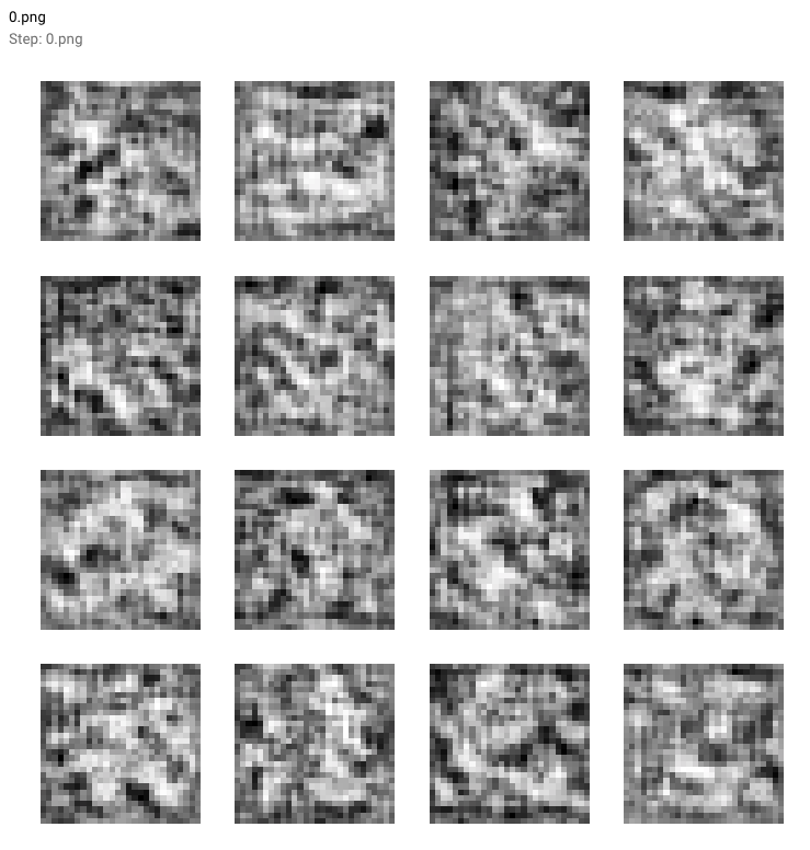
You can see how the Generator models starts off with this fuzzy, grayish output (see 0.png below)that doesn’t really look like the handwritten digits we expect.

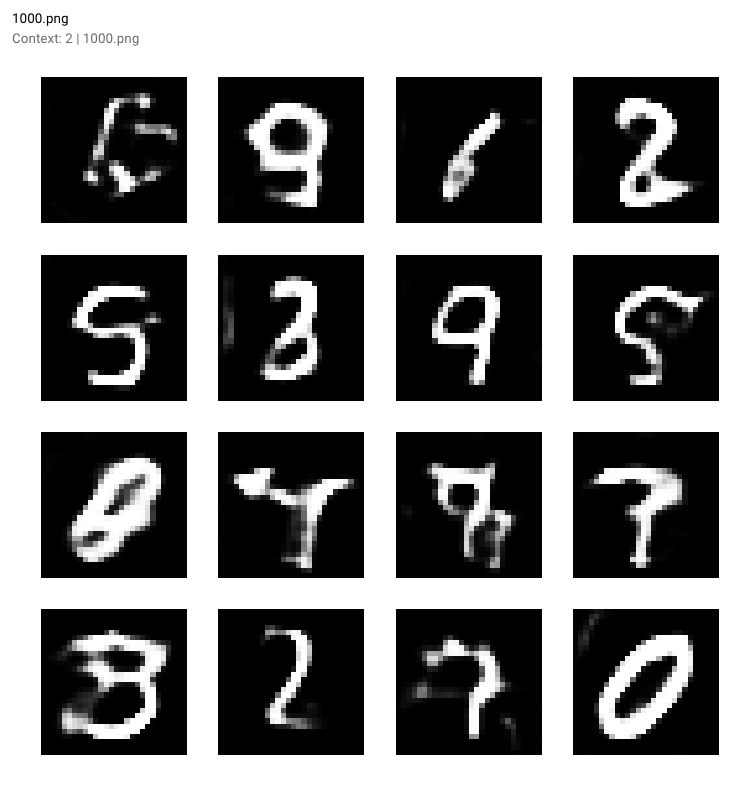
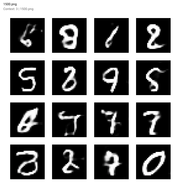
As training progresses and our models’ losses decline, the generated digits become clearer and clear. Check out the generated outputs at:

Step 500:

Step 1000:

Step 1500:

And finally at Step 10,000 — you can see some samples of the GAN-generated digits in the red outlined boxes below

Once our GAN model is done training, we can even review our reported outputs as a movie in Comet’s Graphics tab (just press the play button!).

To complete the experiment, make you sure run experiment.end() to see some summary statistics around the model and GPU usage.

Iterating with your model

 
We could train the model longer to see how that impacts performance, but let’s try iterating with a few different parameters.
Some of the parameters we play around with are:

• the discriminator’s optimizer
• the learning rate
• dropout probability
• batch size

From Wouter’s original blog post, he mentions his own efforts with testing parameters:

I have tested both SGD, RMSprop and Adam for the optimizer of the discriminator but RMSprop performed best. RMSprop is used a low learning rate and I clip the values between -1 and 1. A small decay in the learning rate can help with stabilizing

We’ll try increasing the discriminator’s dropout probability from 0.4 to 0.5 and increasing both the discriminator’s learning rate (from 0.008 to 0.0009) and the generator’s learning rate (from 0.0004 to 0.0006). Easy to see how these changes can get out of hand and difficult to track…🤯

To create a different experiment, simply run the experiment definition cell again and Comet will issue you a new url for your new experiment! It’s nice to keep track of your experiments, so you can compare the differences:

See the difference between the two experiments’ hyperparameters. Can you spot the differences in learning rate and dropout probability that we made?

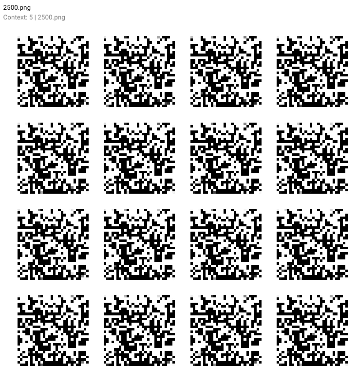
Unfortunately, our adjustments did not improve the model’s performance! In fact, it generated some funky outputs:

That’s it for this tutorial! If you enjoyed this post, feel free to share with a friend who might find it useful 😎

 
Bio: Cecilia Shao is heading Product Growth at comet.ml.

Original. Reposted with permission.

Related:

• MNIST Generative Adversarial Model in Keras
• GANs in TensorFlow from the Command Line: Creating Your First GitHub Project
• Building a Basic Keras Neural Network Sequential Model