Building a Basic Keras Neural Network Sequential Model
The approach basically coincides with Chollet's Keras 4 step workflow, which he outlines in his book "Deep Learning with Python," using the MNIST dataset, and the model built is a Sequential network of Dense layers. A building block for additional posts.
As the title suggest, this post approaches building a basic Keras neural network using the Sequential model API. The specific task herein is a common one (training a classifier on the MNIST dataset), but this can be considered an example of a template for approaching any such similar task.
The approach basically coincides with Chollet's Keras 4 step workflow, which he outlines in his book "Deep Learning with Python," and really amounts to little more than what can be found as an example in the early chapters of the book, or the official Keras tutorials.
The motivation for producing such a post is to use it is a foundational reference for a series of upcoming posts configuring Keras in a variety of different ways. This seemed a better idea than covering the same things over and over again at the start of each post. The content should be useful on its own for those who do not have experience approaching building a neural network in Keras.

Image taken from screenshot of the Keras documentation website
The dataset used is MNIST, and the model built is a Sequential network of Dense layers, intentionally avoiding CNNs for now.
First are the imports and a few hyperparameter and data resizing variables.
from keras import models
from keras.layers import Dense, Dropout
from keras.utils import to_categorical
from keras.datasets import mnist
from keras.utils.vis_utils import model_to_dot
from IPython.display import SVG

import livelossplot
plot_losses = livelossplot.PlotLossesKeras()

NUM_ROWS = 28
NUM_COLS = 28
NUM_CLASSES = 10
BATCH_SIZE = 128
EPOCHS = 10
Next is a function for outputting some simple (but useful) metadata of our dataset. Since we will be using it a few times, it makes sense to put the few lines in a callable function. Reusable code is an end in and of itself :)
def data_summary(X_train, y_train, X_test, y_test):
    """Summarize current state of dataset"""
    print('Train images shape:', X_train.shape)
    print('Train labels shape:', y_train.shape)
    print('Test images shape:', X_test.shape)
    print('Test labels shape:', y_test.shape)
    print('Train labels:', y_train)
    print('Test labels:', y_test)
Next we load our dataset (MNIST, using Keras' dataset utilities), and then use the function above to get some dataset metadata.
# Load data
(X_train, y_train), (X_test, y_test) = mnist.load_data()

# Check state of dataset
data_summary(X_train, y_train, X_test, y_test)
Train images shape: (60000, 28, 28)
Train labels shape: (60000,)
Test images shape: (10000, 28, 28)
Test labels shape: (10000,)
Train labels: [5 0 4 ... 5 6 8]
Test labels: [7 2 1 ... 4 5 6]
To feed MNIST instances into a neural network, they need to be reshaped, from a 2 dimensional image representation to a single dimension sequence. We also convert our class vector to a binary matrix (using to_categorical). This is accomplished below, after which the same function defined above is called again in order to show the effects of our data reshaping.
# Reshape data
X_train = X_train.reshape((X_train.shape[0], NUM_ROWS * NUM_COLS))
X_train = X_train.astype('float32') / 255
X_test = X_test.reshape((X_test.shape[0], NUM_ROWS * NUM_COLS))
X_test = X_test.astype('float32') / 255

# Categorically encode labels
y_train = to_categorical(y_train, NUM_CLASSES)
y_test = to_categorical(y_test, NUM_CLASSES)

# Check state of dataset
data_summary(X_train, y_train, X_test, y_test)
Train images shape: (60000, 784)
Train labels shape: (60000, 10)
Test images shape: (10000, 784)
Test labels shape: (10000, 10)
Train labels: [[0. 0. 0. ... 0. 0. 0.]
 [1. 0. 0. ... 0. 0. 0.]
 [0. 0. 0. ... 0. 0. 0.]
 ...
 [0. 0. 0. ... 0. 0. 0.]
 [0. 0. 0. ... 0. 0. 0.]
 [0. 0. 0. ... 0. 1. 0.]]
Test labels: [[0. 0. 0. ... 1. 0. 0.]
 [0. 0. 1. ... 0. 0. 0.]
 [0. 1. 0. ... 0. 0. 0.]
 ...
 [0. 0. 0. ... 0. 0. 0.]
 [0. 0. 0. ... 0. 0. 0.]
 [0. 0. 0. ... 0. 0. 0.]]
Both of the required data transformations have been accomplished. Now it's time to build, compile, and train a neural network. You can see more about this process in this previous post.
# Build neural network
model = models.Sequential()
model.add(Dense(512, activation='relu', input_shape=(NUM_ROWS * NUM_COLS,)))
model.add(Dropout(0.5))
model.add(Dense(256, activation='relu'))
model.add(Dropout(0.25))
model.add(Dense(10, activation='softmax'))

# Compile model
model.compile(optimizer='rmsprop',
              loss='categorical_crossentropy',
              metrics=['accuracy'])

# Train model
model.fit(X_train, y_train,
          batch_size=BATCH_SIZE,
          epochs=EPOCHS,
          callbacks=[plot_losses],
          verbose=1,
          validation_data=(X_test, y_test))

score = model.evaluate(X_test, y_test, verbose=0)
print('Test loss:', score[0])
print('Test accuracy:', score[1])
The only unorthodox (as far as using the Keras library standalone) step has been the use of the Live Loss Plot callback which outputs epoch-by-epoch loss functions and accuracies at the end of each epoch of training. Make sure you have installed Live Loss Plot prior to running the above code. We are also given the final loss and accuracy on our test dataset.
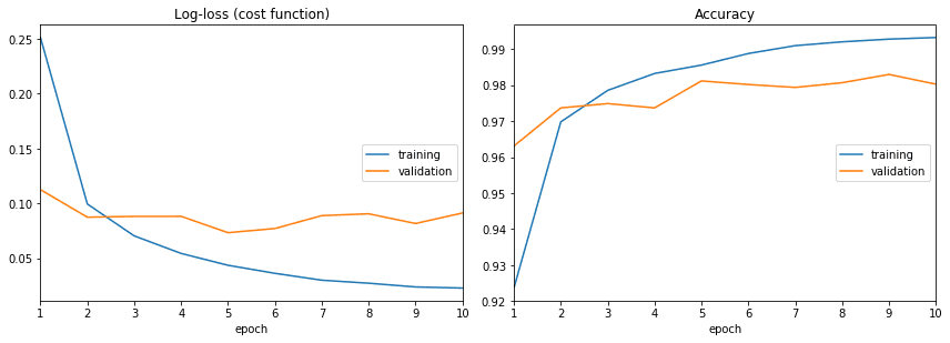
Test loss: 0.09116139834111646
Test accuracy: 0.9803
Almost done, but first let's output a summary of the neural network we built.
# Summary of neural network
model.summary()
Layer (type)                 Output Shape              Param #
=================================================================
dense_1 (Dense)              (None, 512)               401920
_________________________________________________________________
dropout_1 (Dropout)          (None, 512)               0
_________________________________________________________________
dense_2 (Dense)              (None, 256)               131328
_________________________________________________________________
dropout_2 (Dropout)          (None, 256)               0
_________________________________________________________________
dense_3 (Dense)              (None, 10)                2570
=================================================================
Total params: 535,818
Trainable params: 535,818
Non-trainable params: 0
And finally, visualize the model:
# Output network visualization
SVG(model_to_dot(model).create(prog='dot', format='svg'))

The full code is shown below:
As previously stated, this post doesn't cover anything innovative, but we will publish a series of upcoming posts using Keras which hopefully will be more interesting to the reader, and this common starting point should be beneficial for reference.
Also, for those looking for a streamlined approach to building neural networks using the Keras Sequential model, this post should serve as a basic guide to hitting all the important points along the way. What you do after training is up to you (at this point), but we will circle back around to this in the future as well.
Related:
- The Keras 4 Step Workflow
- 7 Steps to Mastering Deep Learning with Keras
- Today I Built a Neural Network During My Lunch Break with Keras