Inside the Mind of a Neural Network with Interactive Code in Tensorflow

By Jae Duk Seo, Ryerson University

GIF from this website

I have been wanting to understand the inner workings of my models, for such a long time. And starting from today, I wish to learn about the topics related to this subject. And for this post I want to cover three topics, histogram of weights, visualizing the activation of neurons, interior / integral gradients.

Please note that this post is for my future self to review these materials.

 

Before Reading On

 

Original Video from TechTalksTV (https://vimeo.com/user72337760) If any problem arises I will delete the video asap. Original video Link here: https://vimeo.com/238242575

This video, is out of scope for this post, but it really helped me to understand Interior and Integral gradient as well as general overview of how can we understand the inner workings of neural network.

 

Data Set / Network Architecture / Accuracy / Class Numbers

 

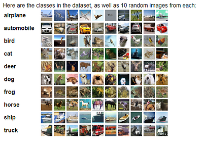
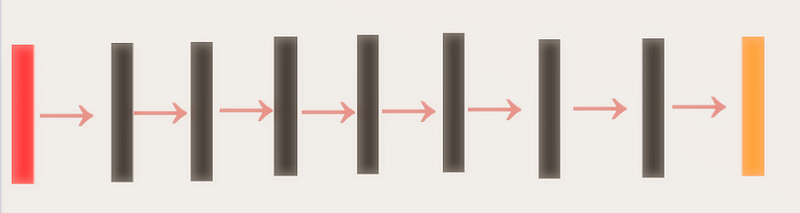
Image from this website

Red Rectangle → Input Image (32*32*3)
Black Rectangle → Convolution with ELU() with / without mean pooling
Orange Rectangle → Softmax for classification

As usual we are going to use the CIFAR 10 data set to train our All Convolutional Network and try to see why the network have predicted certain image into it’s class.

And one thing to note, since this post is more about getting to know the inner workings of the network. I am only going to use 50 images from the test set to measure the accuracy.

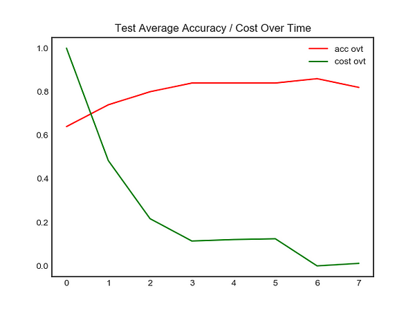
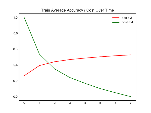
Left Image → Accuracy / Cost over time for Test Image (50 images)
Right Image → Accuracy / Cost over time for Training Image (50000 images)

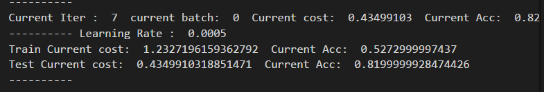
As seen above, the model had a final accuracy of 81 percent, on the 7 epoch. (If you wish to access the full training log, please click here.) Finally, lets take a look at what each number represents for each class.

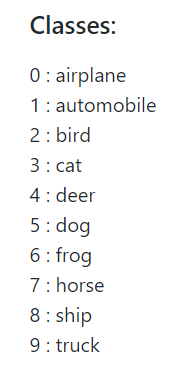
Image from this website

 

Histogram of Weights (Before / After Training )

 

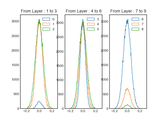
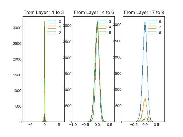
Histogram of weighs before training

Above image is histogram of weights for each layer, for easy visualization I divided into three layers for each histogram. At the very left we can observer the weights generally have a mean value of 0 and standard deviation (stddev) value between 0.04 to 0.06. And this is expected since we declared each layers with different stddev values. Also the reason why some curves are smaller than others is due to different numbers of weights per layers. (e.g. layer 0 only have 3 * 3 * 128 weights, while layer 2 have 3 * 128 * 128 weights.)

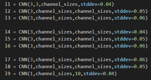
Different stddev values

Histogram of weighs after training

Right off the bat, we can observe a clear difference. especially for the first three layers. The range of the distribution have increase from -5 to 5. However, it seems like most of the weights exist between -1 and 1 (Or close to zero.) For layer 4 to 6, it seems like the mean value have shifted as well as the final three layers.

 

Visualizing the Activation Values for Certain Layers

 

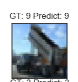
Test Input for the network

Using the technique done by Yosinski and his colleagues, lets visualize how the image above gets modified after layer 3, 6 and 9. (Please note I originally found this method used by Arthur Juliani in this blog post.)

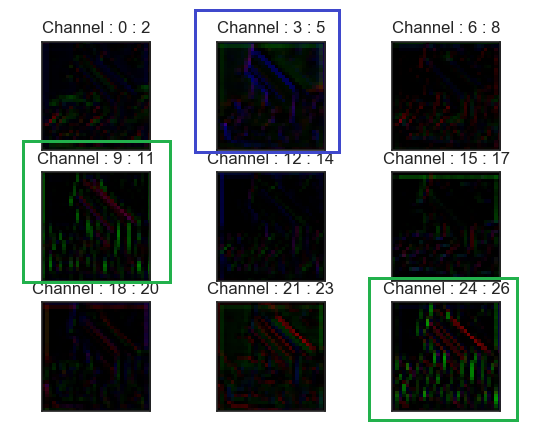
Activation after layer 3

Green Box → Channels where Green Values are captured
Blue Box → Channels where Blue Values are captured

Now there is 128 channels so I won’t visualize them all. Rather I’ll visualize the first 27 channels as seen above. We can see that after layer 3 certain color values gets captured within the network.

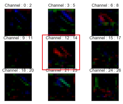
Activation for layer 6

Red Box → Channels where Red Colors are captured

However after the sixth layer, it seems like certain filters are able to capture the color red better than color green or blue.

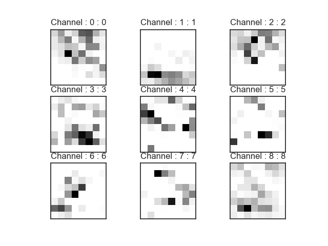
Activation after layer 9

Finally, after ninth layer (right before global average pooling) we can visualize each channel with depth 1 (hence it looks like a gray scale image). However (at least for me), it does not seem to be human intelligible. All images can be found here and I created a GIF accumulating all of the changes.

Order of GIF → Input Image, Activation after Layer 3, Activation After Layer 6, and Activation After Layer 9