3 Main Approaches to Machine Learning Models

 

In September 2018, I published a blog about my forthcoming book on The Mathematical Foundations of Data Science.  The central question we address is: How can we bridge the gap between mathematics needed for Artificial Intelligence (Deep Learning and Machine learning) with that taught in high schools (up to ages 17/18)?

In this post, we present a chapter from this book called “A Taxonomy of Machine Learning Models.” The book is now available for an early bird discount released as chapters. If you are interested in getting early discounted copies, please contact ajit.jaokar at feynlabs.ai.

1. A Taxonomy of Machine Learning Models

There is no simple way to classify machine learning algorithms. In this section, we present a taxonomy of machine learning models adapted from the book Machine Learning by Peter Flach. While the structure for classifying algorithms is based on the book, the explanation presented below is created by us.

For a given problem, the collection of all possible outcomes represents the sample space or instance space.

The basic idea for creating a taxonomy of algorithms is that we divide the instance space by using one of three ways:

• Using a Logical expression.
• Using the Geometry of the instance space.
• Using Probability to classify the instance space.

The outcome of the transformation of the instance space by a machine learning algorithm using the above techniques should be exhaustive (cover all possible outcomes) and mutually exclusive (non-overlapping).

2. Logical models

 

2.1 Logical models - Tree models and Rule models

Logical models use a logical expression to divide the instance space into segments and hence construct grouping models. A logical expression is an expression that returns a Boolean value, i.e., a True or False outcome. Once the data is grouped using a logical expression, the data is divided into homogeneous groupings for the problem we are trying to solve.  For example, for a classification problem, all the instances in the group belong to one class.

There are mainly two kinds of logical models: Tree models and Rule models.

Rule models consist of a collection of implications or IF-THEN rules. For tree-based models, the ‘if-part’ defines a segment and the ‘then-part’ defines the behaviour of the model for this segment. Rule models follow the same reasoning.

Tree models can be seen as a particular type of rule model where the if-parts of the rules are organised in a tree structure. Both Tree models and Rule models use the same approach to supervised learning.  The approach can be summarised in two strategies: we could first find the body of the rule (the concept) that covers a sufficiently homogeneous set of examples and then find a label to represent the body. Alternately, we could approach it from the other direction, i.e., first select a class we want to learn and then find rules that cover examples of the class.

A simple tree-based model is shown below. The tree shows survival numbers of passengers on the Titanic ("sibsp" is the number of spouses or siblings aboard). The values under the leaves show the probability of survival and the percentage of observations in the leaf. The model can be summarised as: Your chances of survival were good if you were (i) a female or (ii) a male younger than 9.5 years with less than 2.5 siblings.

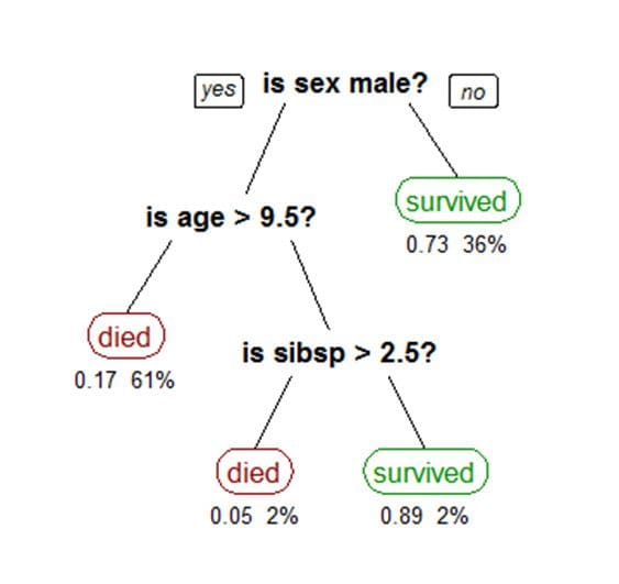
(Image source.)

2.2 Logical models and Concept learning

To understand logical models further, we need to understand the idea of Concept Learning. Concept Learning involves learning logical expressions or concepts from examples. The idea of Concept Learning fits in well with the idea of Machine learning, i.e., inferring a general function from specific training examples. Concept learning forms the basis of both tree-based and rule-based models.  More formally, Concept Learning involves acquiring the definition of a general category from a given set of positive and negative training examples of the category. A Formal Definition for Concept Learning is “The inferring of a Boolean-valued function from training examples of its input and output.” In concept learning, we only learn a description for the positive class and label everything that doesn’t satisfy that description as negative.

The following example explains this idea in more detail.

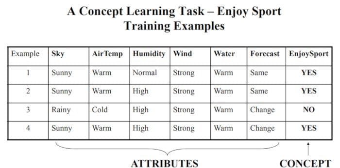
A Concept Learning Task called “Enjoy Sport” as shown above is defined by a set of data from some example days. Each data is described by six attributes. The task is to learn to predict the value of Enjoy Sport for an arbitrary day based on the values of its attribute values. The problem can be represented by a series of hypotheses. Each hypothesis is described by a conjunction of constraints on the attributes. The training data represents a set of positive and negative examples of the target function. In the example above, each hypothesis is a vector of six constraints, specifying the values of the six attributes –  Sky, AirTemp, Humidity, Wind, Water, and Forecast. The training phase involves learning the set of days (as a conjunction of attributes) for which Enjoy Sport = yes.

Thus, the problem can be formulated as:

• Given instances X  which represent a set of all possible days, each described by the attributes:
  • Sky – (values: Sunny, Cloudy, Rainy),
  • AirTemp – (values: Warm, Cold),
  • Humidity – (values: Normal, High),
  • Wind – (values: Strong, Weak),
  • Water – (values: Warm, Cold),
  • Forecast – (values: Same, Change).

Try to identify a function that can predict the target variable Enjoy Sport as yes/no, i.e., 1 or 0.

2.3 Concept learning as a search problem and as Inductive Learning

We can also formulate Concept Learning as a search problem. We can think of  Concept learning as searching through a set of predefined space of potential hypotheses to identify a hypothesis that best fits the training examples.  Concept learning is also an example of Inductive Learning. Inductive learning, also known as discovery learning, is a process where the learner discovers rules by observing examples. Inductive learning is different from deductive learning, where students are given rules that they then need to apply. Inductive learning is based on the inductive learning hypothesis. The Inductive Learning Hypothesis postulates that: Any hypothesis found to approximate the target function well over a sufficiently large set of training examples is expected to approximate the target function well over other unobserved examples.  This idea is the fundamental assumption of inductive learning.

To summarise, in this section, we saw the first class of algorithms where we divided the instance space based on a logical expression. We also discussed how logical models are based on the theory of concept learning – which in turn – can be formulated as an inductive learning or a search problem.

3. Geometric models

In the previous section, we have seen that with logical models, such as decision trees, a logical expression is used to partition the instance space. Two instances are similar when they end up in the same logical segment. In this section, we consider models that define similarity by considering the geometry of the instance space.  In Geometric models, features could be described as points in two dimensions (x- and y-axis) or a three-dimensional space (x, y, and z). Even when features are not intrinsically geometric, they could be modelled in a geometric manner (for example, temperature as a function of time can be modelled in two axes). In geometric models, there are two ways we could impose similarity.

• We could use geometric concepts like lines or planes to segment (classify) the instance space. These are called Linear models.
• Alternatively, we can use the geometric notion of distance to represent similarity. In this case, if two points are close together, they have similar values for features and thus can be classed as similar. We call such models as Distance-based models.

3.1 Linear models

Linear models are relatively simple. In this case, the function is represented as a linear combination of its inputs. Thus, if x₁ and x₂ are two scalars or vectors of the same dimension and a and b are arbitrary scalars, then ax₁ + bx₂ represents a linear combination of x₁ and x₂. In the simplest case where f(x) represents a straight line, we have an equation of the form f (x) = mx + c where c represents the intercept and m represents the slope.

 

(Image source.)

Linear models are parametric, which means that they have a fixed form with a small number of numeric parameters that need to be learned from data. For example, in f (x) = mx + c, m and c are the parameters that we are trying to learn from the data. This technique is different from tree or rule models, where the structure of the model (e.g., which features to use in the tree, and where) is not fixed in advance.

Linear models are stable, i.e., small variations in the training data have only a limited impact on the learned model. In contrast, tree models tend to vary more with the training data, as the choice of a different split at the root of the tree typically means that the rest of the tree is different as well.  As a result of having relatively few parameters, Linear models have low variance and high bias. This implies that Linear models are less likely to overfit the training data than some other models. However, they are more likely to underfit. For example, if we want to learn the boundaries between countries based on labelled data, then linear models are not likely to give a good approximation.

In this section, we could also use algorithms that include kernel methods, such as support vector machine (SVM). Kernel methods use the kernel function to transform data into another dimension where easier separation can be achieved for the data, such as using a hyperplane for SVM.

3.2 Distance-based models

Distance-based models are the second class of Geometric models. Like Linear models, distance-based models are based on the geometry of data. As the name implies, distance-based models work on the concept of distance.  In the context of Machine learning, the concept of distance is not based on merely the physical distance between two points. Instead, we could think of the distance between two points considering the mode of transport between two points. Travelling between two cities by plane covers less distance physically than by train because a plane is unrestricted. Similarly, in chess, the concept of distance depends on the piece used – for example, a Bishop can move diagonally.   Thus, depending on the entity and the mode of travel, the concept of distance can be experienced differently. The distance metrics commonly used are Euclidean, Minkowski, Manhattan, and Mahalanobis.

(Image source.)

Distance is applied through the concept of neighbours and exemplars. Neighbours are points in proximity with respect to the distance measure expressed through exemplars. Exemplars are either centroids that find a centre of mass according to a chosen distance metric or medoids that find the most centrally located data point. The most commonly used centroid is the arithmetic mean, which minimises squared Euclidean distance to all other points.

Notes:

• The centroid represents the geometric centre of a plane figure, i.e., the arithmetic mean position of all the points in the figure from the centroid point. This definition extends to any object in n-dimensional space: its centroid is the mean position of all the points.
• Medoids are similar in concept to means or centroids. Medoids are most commonly used on data when a mean or centroid cannot be defined. They are used in contexts where the centroid is not representative of the dataset, such as in image data.

Examples of distance-based models include the nearest-neighbour models, which use the training data as exemplars – for example, in classification. The K-means clustering algorithm also uses exemplars to create clusters of similar data points.

4. Probabilistic models

The third family of machine learning algorithms is the probabilistic models. We have seen before that the k-nearest neighbour algorithm uses the idea of distance (e.g., Euclidian distance) to classify entities, and logical models use a logical expression to partition the instance space. In this section, we see how the probabilistic models use the idea of probability to classify new entities.

Probabilistic models see features and target variables as random variables. The process of modelling represents and manipulates the level of uncertainty with respect to these variables. There are two types of probabilistic models: Predictive and Generative. Predictive probability models use the idea of a conditional probability distribution P (Y |X) from which Y can be predicted from X.  Generative models estimate the joint distribution P (Y, X).  Once we know the joint distribution for the generative models, we can derive any conditional or marginal distribution involving the same variables. Thus, the generative model is capable of creating new data points and their labels, knowing the joint probability distribution. The joint distribution looks for a relationship between two variables. Once this relationship is inferred, it is possible to infer new data points.

Naïve Bayes is an example of a probabilistic classifier.

The goal of any probabilistic classifier is given a set of features (x_0 through x_n) and a set of classes (c_0 through c_k), we aim to determine the probability of the features occurring in each class, and to return the most likely class. Therefore, for each class, we need to calculate P(c_i | x_0, …, x_n).

We can do this using the Bayes rule defined as

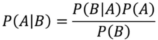
The Naïve Bayes algorithm is based on the idea of Conditional Probability.  Conditional probability is based on finding the probability that something will happen, given that something else has already happened. The task of the algorithm then is to look at the evidence and to determine the likelihood of a specific class and assign a label accordingly to each entity.

Conclusion

The above discussion presents a way to classify algorithms based on their mathematical foundations. While the discussion is simplified, it provides a comprehensive way to explore algorithms from first principles. If you are interested in getting early discounted copies, please contact ajit.jaokar at feynlabs.ai.

Related:

• Decision Trees — An Intuitive Introduction
• A Beginner’s Guide to Linear Regression in Python with Scikit-Learn
• Naive Bayes from Scratch using Python only – No Fancy Frameworks