Optimization with Python: How to make the most amount of money with the least amount of risk?

comments

Introduction

One of the major goals of the modern enterprise of data science and analytics is to solve complex optimization problems for business and technology companies to maximize their profit.

In my article “Linear Programming and Discrete Optimization with Python,” we touched on basic discrete optimization concepts and introduced a Python library PuLP for solving such problems.

Although a linear programming (LP) problem is defined only by linear objective function and constraints, it can be applied to a surprisingly wide variety of problems in diverse domains ranging from healthcare to economics, business to military.

In this article, we show one such amazing application of LP using Python programming in the area of economic planning — maximizing the expected profit from a stock market investment portfolio while minimizing the risk associated with it.

Sounds interesting? Please read on.

How to maximize profit and minimize risk in the stock market?

The 1990 Nobel prize in Economics went to Harry Markowitz, acknowledged for his famous Modern Portfolio Theory (MPT), as it is known in the parlance of financial markets. The original paper was published long back in 1952.

Source: AZ Quotes

The key word here is Balanced.

A good, balanced portfolio must offer both protections (minimizing the risk) and opportunities (maximizing profit).

And, when concepts such as minimization and maximization are involved, it is natural to cast the problem in terms of mathematical optimization theory.

The fundamental idea is rather simple and is rooted in the innate human nature of risk aversion.

In general, stock market statistics show that higher risk is associated with a greater probability of higher return and lower risk with a greater probability of smaller return.

MPT assumes that investors are risk-averse, meaning that given two portfolios that offer the same expected return, investors will prefer the less risky one. Think about it. You will collect high-risk stocks only if they carry a high probability of large return percentage.

But how to quantify the risk? It is a murky concept for sure and can mean different things to different people. However, in the generally accepted economic theory, the variability (volatility) of a stock price (defined over a fixed time horizon) is equated with risk.

Therefore, the central optimization problem is to minimize the risk while ensuring a certain amount of return in profits. Or, maximizing the profit while keeping the risk below a certain threshold.

An example problem

In this article, we will show a very simplified version of the portfolio optimization problem, which can be cast into an LP framework and solved efficiently using simple Python scripting.

The goal is to illustrate the power and possibility of such optimization solvers for tackling complex real-life problems.

We work with 24 months stock price (monthly average) for three stocks — Microsoft, Visa, Walmart. These are older data, but they demonstrate the process flawlessly.

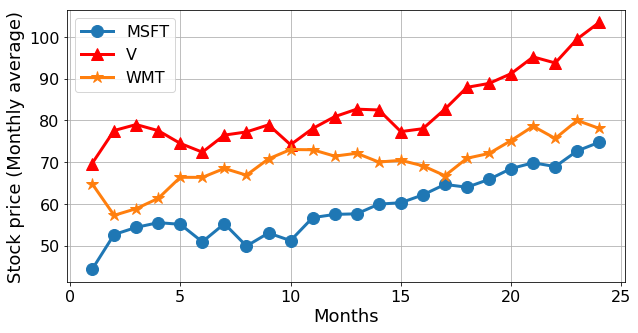
Fig: Monthly stock price of three companies over a certain 24-month period.

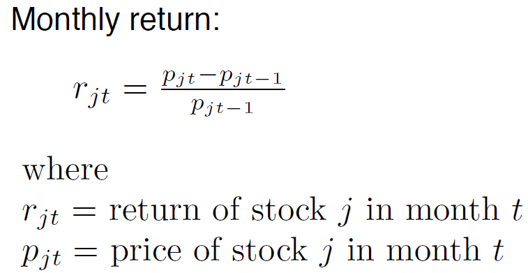
How to define the return? We can simply compute a rolling monthly return by subtracting the previous month’s average stock price from the current month and dividing by the previous month’s price.

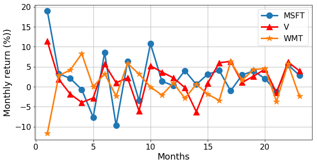
The return is shown in the following figure,

The optimization model

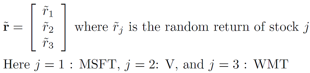
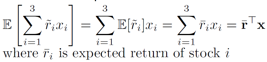
The return on a stock is an uncertain quantity. We can model it as a random vector.

The portfolio can also be modeled as a vector.

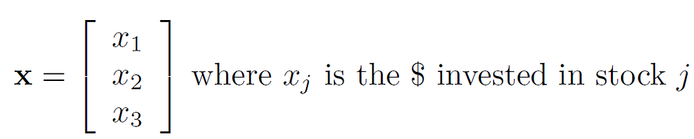
Therefore, the return on a certain portfolio is given by an inner product of these vectors, and it is a random variable. The million-dollar question is:

How can we compare random variables (corresponding to different portfolios) to select a “best” portfolio?

Following the Markowitz model, we can formulate our problem as,

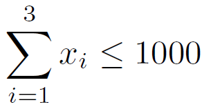
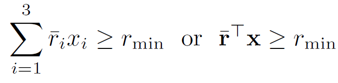
Given a fixed quantity of money (say $1000), how much should we invest in each of the three stocks so as to (a) have a one month expected return of at least a given threshold, and (b) minimize the risk (variance) of the portfolio return.

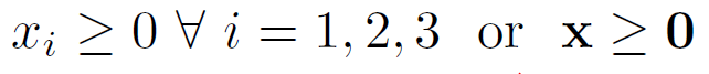
We cannot invest a negative quantity. This is the non-negativity constraint,

Assuming no transaction cost, the total investment is restricted by the fund at hand,

Return on the investment,

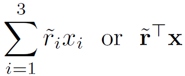
But this is a random variable. So, we have to work with the expected quantities,

Supposed we want a minimum expected return. Therefore,

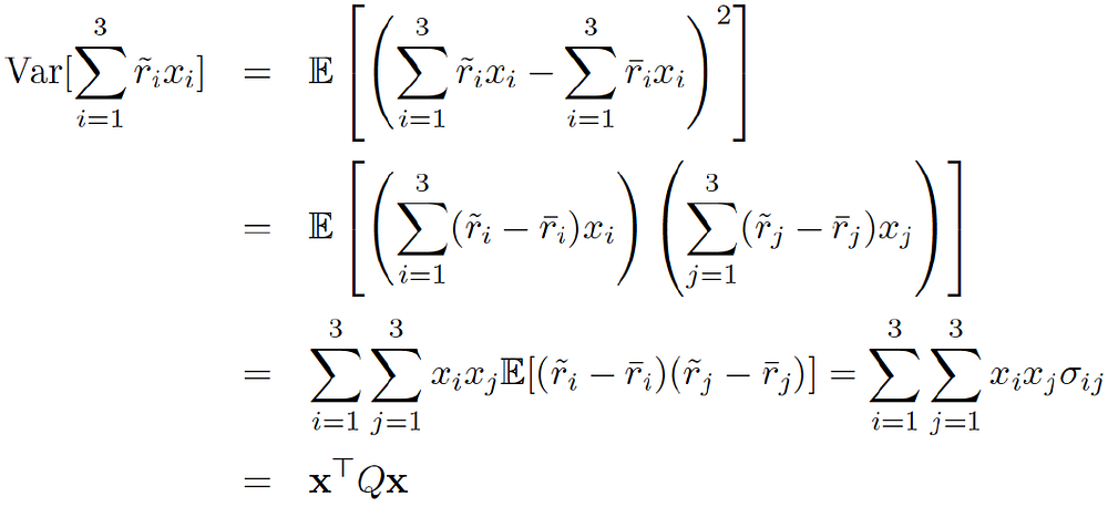
Now, to model the risk, we have to compute the variance,

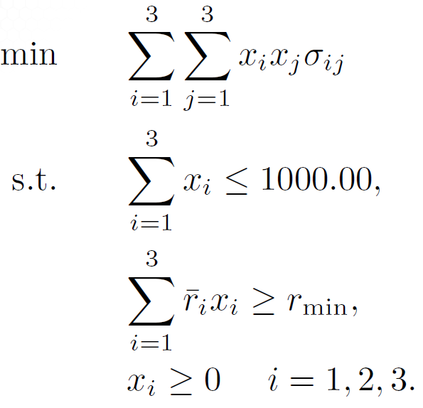
Putting together, the final optimization model is,

Next, we show how easy it is to formulate and solve this problem using a popular Python library.

Using Python to solve the optimization: CVXPY

The library we are going to use for this problem is called CVXPY. It is a Python-embedded modeling language for convex optimization problems. It allows you to express your problem in a natural way that follows the mathematical model, rather than in the restrictive standard form required by solvers.

The entire code is given in this Jupyter notebook. Here, I just show the core code snippets.

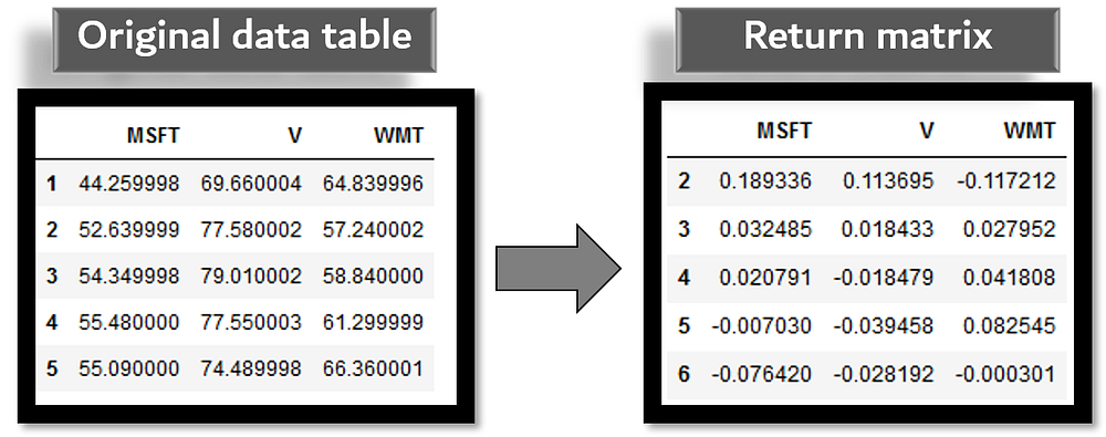
To set up the necessary data, the key is to compute the return matrix from the data-table of the monthly price. The code is given below,

import numpy as np
import pandas as pd
from cvxpy import *

mp = pd.read_csv("monthly_prices.csv",index_col=0)
mr = pd.DataFrame()

# compute monthly returns
for s in mp.columns:
    date = mp.index[0]
    pr0 = mp[s][date] 
    for t in range(1,len(mp.index)):
        date = mp.index[t]
        pr1 = mp[s][date]
        ret = (pr1-pr0)/pr0
        mr.set_value(date,s,ret)
        pr0 = pr1

Now, if you view the original data table and the return table side by side, it looks like following,

Next, we simply compute the mean (expected) return and the covariance matrix from this return matrix,

# Mean return
r = np.asarray(np.mean(return_data, axis=1))

# Covariance matrix
C = np.asmatrix(np.cov(return_data))

After that, CVXPY allows setting up the problem simply following the mathematical model we constructed above,

# Get symbols
symbols = mr.columns

# Number of variables
n = len(symbols)

# The variables vector
x = Variable(n)

# The minimum return
req_return = 0.02

# The return
ret = r.T*x

# The risk in xT.Q.x format
risk = quad_form(x, C)

# The core problem definition with the Problem class from CVXPY
prob = Problem(Minimize(risk), [sum(x)==1, ret >= req_return, x >= 0])

Note the use of extremely useful classes like quad_form() and Problem()from the CVXPY framework.

Voila!

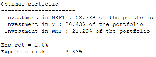
We can write a simple code to solve the Problem and show the optimal investment quantities which ensure a minimum return of 2% while also keeping the risk at a minimum.

try:
    prob.solve()
    print ("Optimal portfolio")
    print ("----------------------")
    for s in range(len(symbols)):
       print (" Investment in {} : {}% of the portfolio".format(symbols[s],round(100*x.value[s],2)))
    print ("----------------------")
    print ("Exp ret = {}%".format(round(100*ret.value,2)))
    print ("Expected risk    = {}%".format(round(100*risk.value**0.5,2)))
except:
    print ("Error")

The final result is given by,

Extending the problem

Needless to say that the setup and simplifying assumptions of our model can make this problem sound simpler than what it is. But once you understand the basic logic and the mechanics of solving such an optimization problem, you can extend it to multiple scenarios,

• Hundreds of stocks, longer time horizon data
• Multiple risk/return ratio and threshold
• Minimize risk or maximize return (or both)
• Investing in a group of companies together
• Either/or scenario — invest either in Cococola or in Pepsi but not in both

You have to construct more complicated matrices and a longer list of constraints, use indicator variables to turn this into a mixed-integer problem - but all of these are inherently supported by packages like CVXPY.

Look at the examples page of the CVXPY package to know about the breadth of optimization problems that can be solved using the framework.

Summary

In this article, we discussed how the key concepts from a seminal economic theory could be used to formulate a simple optimization problem for stock market investment.

For illustration, we took a sample dataset of three companies’ average monthly stock price and showed how a linear programming model could be set up in no time using basic Python data science libraries such as NumPy, Pandas, and an optimization framework called CVXPY.

Having a working knowledge of such flexible and powerful packages adds immense value to the skillset of upcoming data scientists because the need for solving optimization problems arise in all facets of science, technology, and business problems.

Readers are encouraged to try more complex versions of this investment problem for fun and learning.

Original. Reposted with permission.

Bio: Tirthajyoti Sarkar is the Senior Principal Engineer at ON Semiconductor working on Deep Learning/Machine Learning based design automation projects.

Related:

• Data Analytics Models in Quantitative Finance and Risk Management
• How Optimization Works
• Linear Programming and Discrete Optimization with Python using PuLP