Linear Programming and Discrete Optimization with Python using PuLP

comments

Introduction

Discrete optimization is a branch of optimization methodology which deals with discrete quantities i.e. non-continuous functions. It is quite ubiquitous in as diverse applications such as financial investment, diet planning, manufacturing processes, and player or schedule selection for professional sports.

Linear and (mixed) integer programming are techniques to solve problems which can be formulated within the framework of discrete optimization.

Knowledge of such optimization techniques is extremely useful for data scientists and machine learning (ML) practitioners as discrete and continuous optimization lie at the heart of modern ML and AI systems as well as data-driven business analytics processes.

There are many commercial optimizer tools, but having hands-on experience with a programmatic way of doing optimization is invaluable.

There is a long and rich history of the theoretical development of robust and efficient solvers for optimization problems. However, focusing on practical applications, we will skip that history and move straight to the part of learning how to use programmatic tools to formulate and solve such optimization problems.

There are many excellent optimization packages in Python. In this article, we will specifically talk about PuLP. But before going to the Python library, let us get a sense of the kind of problem we can solve with it.

An example problem (or two)

Suppose you are in charge of the diet plan for high school lunch. Your job is to make sure that the students get the right balance of nutrition from the chosen food.

However, there are some restrictions in terms of budget and the variety of food that needs to be in the diet to make it interesting. The following table shows, in detail, the complete nutritional value for each food item, and their maximum/minimum daily intake.

The discrete optimization problem is simple: Minimize the cost of the lunch given these constraints (on total calories but also on each of the nutritional component e.g. cholesterol, vitamin A, calcium, etc.

Essentially, in a casual mathematical language, the problem is,

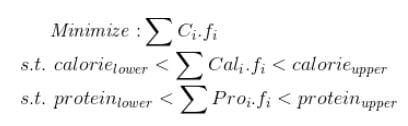
Notice that the inequality relations are all linear in nature i.e. the variables f are multiplied by constant coefficients and the resulting terms are bounded by constant limits and that’s what makes this problem solvable by an LP technique.

You can imagine that this kind of problem may pop up in business strategy extremely frequently. Instead of nutritional values, you will have profits and other types of business yields, and in place of price/serving, you may have project costs in thousands of dollars. As a manager, your job will be to choose the projects, that give maximum return on investment without exceeding a total budget of funding the project.

Similar optimization problem may crop up in a factory production plan too, where maximum production capacity will be functions of the machines used and individual products will have various profit characteristics. As a production engineer, your job could be to assign machine and labor resources carefully to maximize the profit while satisfying all the capacity constraints.

Fundamentally, the commonality between these problems from disparate domains is that they involve maximizing or minimizing a linear objective function, subject to a set of linear inequality or equality constraints.

For the diet problem, the objective function is the total cost which we are trying to minimize. The inequality constraints are given by the minimum and maximum bounds on each of the nutritional components.

PuLP — a Python library for linear optimization

There are many libraries in the Python ecosystem for this kind of optimization problems. PuLP is an open-source linear programming (LP) package which largely uses Python syntax and comes packaged with many industry-standard solvers. It also integrates nicely with a range of open source and commercial LP solvers.
You can install it using pip (and also some additional solvers)

$ sudo pip install pulp            # PuLP
$ sudo apt-get install glpk-utils  # GLPK
$ sudo apt-get install coinor-cbc  # CoinOR

Detailed instructions about installation and testing are here. Then, just import everything from the library.

from pulp import *

See a nice video on solving linear programming here.

How to formulate the optimization problem?

First, we create a LP problem with the method LpProblemin PuLP.

prob = LpProblem("Simple Diet Problem",LpMinimize)

Then, we need to create bunches of Python dictionary objects with the information we have from the table. The code is shown below,

# Read the first few rows dataset in a Pandas DataFrame
# Read only the nutrition info not the bounds/constraints
df = pd.read_excel("diet - medium.xls",nrows=17)

# Create a list of the food items
food_items = list(df['Foods'])

# Create a dictinary of costs for all food items
costs = dict(zip(food_items,df['Price/Serving']))

# Create a dictionary of calories for all food items
calories = dict(zip(food_items,df['Calories']))

# Create a dictionary of total fat for all food items
fat = dict(zip(food_items,df['Total_Fat (g)']))

# Create a dictionary of carbohydrates for all food items
carbs = dict(zip(food_items,df['Carbohydrates (g)']))

For brevity, we did not show the full code here. You can take all the nutrition components and create separate dictionaries for them.

Then, we create a dictionary of food items variables with lower bound =0 and category continuous i.e. the optimization solution can take any real-numbered value greater than zero.

Note the particular importance of the lower bound.

In our mind, we cannot think a portion of food anything other than a non-negative, finite quantity but the mathematics does not know this.

Without an explicit declaration of this bound, the solution may be non-sensical as the solver may try to come up with negative quantities of food choice to reduce the total cost while still meeting the nutrition requirement!

food_vars = LpVariable.dicts("Food",food_items,lowBound=0,cat='Continuous')

Next, we start building the LP problem by adding the main objective function. Note the use of thelpSum method.

prob += lpSum([costs[i]*food_vars[i] for i in food_items])

We further build on this by adding calories constraints,

prob += lpSum([calories[f] * food_vars[f] for f in food_items]) >= 800.0
prob += lpSum([calories[f] * food_vars[f] for f in food_items]) <= 1300.0

We can pile up all the nutrition constraints. For simplicity, we are just adding four constraints on fat, carbs, fiber, and protein. The code is shown below,

# Fat
prob += lpSum([fat[f] * food_vars[f] for f in food_items]) >= 20.0, "FatMinimum"
prob += lpSum([fat[f] * food_vars[f] for f in food_items]) = 130.0, "CarbsMinimum"
prob += lpSum([carbs[f] * food_vars[f] for f in food_items]) = 60.0, "FiberMinimum"
prob += lpSum([fiber[f] * food_vars[f] for f in food_items]) = 100.0, "ProteinMinimum"
prob += lpSum([protein[f] * food_vars[f] for f in food_items]) <= 150.0, "ProteinMaximum"

And we are done with formulating the problem!

In any optimization scenario, the hard part is the formulation of the problem in a structured manner which is presentable to a solver.

We have done the hard part. Now, it is the relatively easier part of running a solver and examining the solution.