 5 Probability Distributions Every Data Scientist Should Know
 5 Probability Distributions Every Data Scientist Should Know
Having an understanding of probability distributions should be a priority for data scientists. Make sure you know what you should by reviewing this post on the subject.
Probability Distributions are like 3D glasses. They allow a skilled Data Scientist to recognize patterns in otherwise completely random variables.
In a way, most of the other Data Science or Machine Learning skills are based on certain assumptions about the probability distributions of your data.
This makes probability knowledge part of the basis on which you can build your toolkit as a statistician. The first steps if you are figuring out how to become a Data Scientist.
Without further ado, let us cut to the chase.
What are Probability Distributions?
In Probability and Statistics, a random variable is a thing that takes random values, like “the height of the next person I see” or “the amount of cook’s hairs in my next ramen bowl”.
Given a random variable X, we’d like to have a way of describing which values it takes. Even more than that, we’d like to characterize how likely it is for that variable to take a certain value x.
For instance, if X is “how many cats my girlfriend has”, then there’s a non-zero chance that number could be 1. One could argue there’s a non-zero probability that value could even be 5 or 10.
However, there’s no way (and therefore no probability) that a person will have negative cats.
We therefore would like an unambiguous, mathematical way of expressing every possible value x a variable X can take, and how likely the event (X= x) is.
In order to do this, we define a function P, such that P(X = x) is the probability of the variable X having a value of x.
We could also ask for P(X < x), or P(X > x), for intervals instead of discrete values. This will become even more relevant soon.
P is the variable’s density function, and it characterizes that variable’s distribution.
Over time, scientists have come to realize many things in nature and real life tend to behave similarly, with variables sharing a distribution, or having the same density functions (or a similar function changing a few constants in it).
Interestingly, for P to be an actual density function, some things have to apply.
- P(X =x) <= 1 for any value x. Nothing’s more certain than certain.
- P(X =x) >= 0 for any value x. A thing can be impossible, but not less likely than that.
- And the last one: the sum of P(X=x) for all possible values x is 1.
This last one means something like “the probability of X taking any value in the universe, has to add up to 1, since we know it will take some value”.
Discrete vs Continuous Random Variable Distributions
Lastly, random variables can be thought of as belonging to two groups: discrete and continuous random variables.
Discrete Random Variables
Discrete variables have a discrete set of possible values, each of them with a non-zero probability.
For instance, when flipping a coin, if we say
X = “1 if the coin is heads, 0 if tails”
Then P(X = 1) = P(X = 0) = 0.5.
Note however, that a discrete set need not be finite.
A geometric distribution, is used for modelling the chance of some event with probability p happening after k retries.
It has the following density formula.

Where k can take any non-negative value with a positive probability.
Notice how the sum of all possible values’ probabilities still adds up to 1.
Continuous Random Variables
If you said
X = “the length in millimeters (without rounding) of a randomly plucked hair from my head”
Which possible values can X take? We can all probably agree a negative value doesn’t make any sense here.
However if you said it is exactly 1 millimeter, and not 1.1853759… or something like that, I would either doubt your measuring skills, or your measuring error reporting.
A continuous random variable can take any value in a given (continuous) interval.
Therefore, if we assigned a non-zero probability to all of its possible values, their sum would not add up to 1.
To solve this, if X is continuous, we set P(X=x) = 0 for all k, and instead assign a non-zero chance to X taking a value in a certain interval.
To express the probability of X laying between values a and b, we say P(a < X < b).
Instead of just replacing values in a density function, to get P(a < X < b) for X a continuous variable, you’ll integrate X‘s density function from a to b.
Whoah, you’ve made it through the whole theory section! Here’s your reward.

Reward puppy. Source: Pixabay.
Now that you know what a probability distribution is, let’s learn about some of the most common ones!
Bernoulli Probability Distribution
A Random Variable with a Bernoulli Distribution is among the simplest ones.
It represents a binary event: “this happened” vs “this didn’t happen”, and takes a value pas its only parameter, which represents the probability that the event will occur.
A random variable B with a Bernoulli distribution with parameter p will have the following density function:
P(B = 1) = p, P(B =0)= (1-p)
Here B=1 means the event happened, and B=0 means it didn’t.
Notice how both probabilities add up to 1, and therefore no other value for B will be possible.
Uniform Probability Distribution
There are two kinds of uniform random variables: discrete and continuous ones.
A discrete uniform distribution will take a (finite) set of values S, and assign a probability of 1/n to each of them, where n is the amount of elements in S.
This way, if for instance my variable Y was uniform in {1,2,3}, then there’d be a 33% chance each of those values came out.
A very typical case of a discrete uniform random variable is found in dice, where your typical dice has the set of values {1,2,3,4,5,6}.
A continuous uniform distribution, instead, only takes two values a and b as parameters, and assigns the same density to each value in the interval between them.
That means the probability of Y taking a value in an interval (from c to d) is proportional to its size versus the size of the whole interval (b-a).
Therefore if Y is uniformly distributed between a and b, then

This way, if Y is a uniform random variable between 1 and 2,
P(1 < X < 2)=1 and P(1 < X < 1.5) = 0.5
Python’s random package’s random method samples a uniformly distributed continuous variable between 0 and 1.
Interestingly, it can be shown that any other distribution can be sampled given a uniform random values generator and some calculus.
Normal Probability Distributions
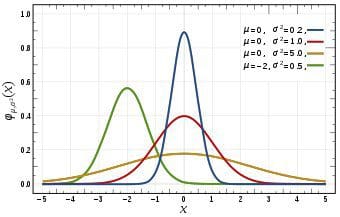
Normal Distributions. source: Wikipedia
Normally distributed variables are so commonly found in nature, they’re actually the norm. That’s actually where the name comes from.
If you round up all your workmates and measure their heights, or weigh them all and plot a histogram with the results, odds are it’s gonna approach a normal distribution.
I actually saw this effect when I showed you Exploratory Data Analysis examples.
It can also be shown that if you take a sample of any random variable and average those measures, and repeat that process many times, that average will also have a normal distribution. That fact’s so important, it’s called the fundamental theorem of statistics.
Normally distributed variables:
- Are symmetrical, centered around a mean (usually called μ).
- Can take all values on the real space, but only deviate two sigmas from the norm 5% of the time.
- Are literally everywhere.
Most often if you measure any empirical data and it’s symmetrical, assuming it’s normal will kinda work.
For example, rolling K dice and adding up the results will distribute pretty much normally.
Log-Normal Probability Distribution
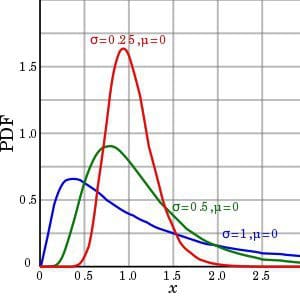
Lognormal distribution. source: Wikipedia
Log-normal probability distribution is Normal Probability Distribution’s smaller, less frequently seen sister.
A variable X is said to be log-normally distributed if the variable Y = log(X) follows a normal distribution.
When plotted in a histogram, log-normal probability distributions are asymmetrical, and become even more so if their standard deviation is bigger.
I believe lognormal distributions to be worth mentioning, because most money-based variables behave this way.
If you look at the probability distributions of any variable that relates to money, like
- Amount sent on the latest transfer of a certain bank.
- Volume of the latest transaction in Wall Street.
- A set of companies’ quarterly earnings for a given quarter.
They will usually not have a normal probability distribution, but will behave much closer to a lognormal random variable.
(For other Data Scientists: chime in in the comments if you can think of any other empirical lognormal variables you’ve come across in your work! Especially anything outside of finances).
Exponential Probability Distribution
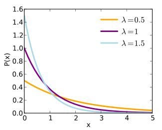
Exponential distribution. source: Wikipedia
Exponential probability distributions appear everywhere, too.
They are heavily linked to a Probability concept called a Poisson Process.
Stealing straight from Wikipedia, a Poisson Process is “a process in which events occur continuously and independently at a constant average rate“.
All that means is, if:
- You have a lot of events going.
- They happen at a certain rate (which does not change over time).
- Just because one happened the chances of another one happening don’t change.
Then you have a Poisson process.
Some examples could be requests coming to a server, transactions happening in a supermarket, or birds fishing in a certain lake.
Imagine a Poisson Process with a frequency rate of λ (say, events happen once every second).
Exponential random variables model the time it takes, after an event, for the next event to occur.
Interestingly, in a Poisson Process an event can happen anywhere between 0 and infinity times (with decreasing probability), in any interval of time.
This means there’s a non-zero chance that the event won’t happen, no matter how long you wait. It also means it could happen a lot of times in a very short interval.
In class we used to joke bus arrivals are Poisson Processes. I think the response time when you send a WhatsApp message to some people also fits the criteria.
However, the λ parameter regulates the frequency of the events.
It will make the expected time it actually takes for an event to happen center around a certain value.
This means if we know a taxi passes our block every 15 minutes, even though theoretically we could wait for it forever, it’s extremely likely we won’t wait longer than, say, 30 minutes.
Exponential Probability Distribution In Data Science
Here’s the density function for an exponential distribution random variable:

Suppose you have a sample from a variable and want to see if it can be modelled with an Exponential distribution Variable.
The optimum λ parameter can be easily estimated as the inverse of the average of your sampled values.
Exponential variables are very good for modelling any probability distributions with very infrequent, but huge (and mean-breaking) outliers.
This is because they can take any non-negative value but center in smaller ones, with decreased frequency as the value grows.
In a particularly outlier-heavy sample, you may want to estimate λ as the median instead of the average, since the median is more robust to outliers. Your mileage may vary on this one, so take it with a grain of salt.
Conclusions
To sum up, as Data Scientists, I think it’s important for us to learn the basics.
Probability and Statistics may not be as flashy as Deep Learning or Unsupervised Machine Learning, but they are the bedrock of Data Science. Especially Machine Learning.
Feeding a Machine Learning model with features without knowing which distribution they follow is, in my experience, a poor choice.
It’s also good to remember the ubiquity of Exponential and Normal Probability Distributions, and their smaller counterpart, the lognormal distribution.
Knowing their properties, uses and appearance is game-changing when training a Machine Learning model. It’s also generally good to keep them in mind while doing any kind of Data Analysis.
Did you find any part of this article useful? Was it all stuff you already knew? did you learn anything new? Let me know in the comments!
Contact me on Twitter, Medium of dev.to if there’s anything you don’t think was clear enough, anything that you disagree with, or just anything that’s plain wrong. Don’t worry, I don’t bite.
Bio: Luciano Strika is a computer science student at Buenos Aires University, and a data scientist at MercadoLibre. He also writes about machine learning and data on www.datastuff.tech.
Original. Reposted with permission.
Related:
- Data Science Basics: Power Laws and Distributions
- Basic Statistics in Python: Probability
- Probability Mass and Density Functions