 11 Important Probability Distributions Explained
 11 Important Probability Distributions Explained
There are many distribution functions considered in statistics and machine learning, which can seem daunting to understand at first. Many are actually closely related, and with these intuitive explanations of the most important probability distributions, you can begin to appreciate the observations of data these distributions communicate.
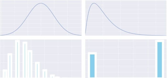
Image Created by Author.
Probability distributions were so daunting when I first saw them, partly because there are so many of them, and they all have such unfamiliar names.
Fast forward to today, and I realized that they’re actually very simple concepts to understand when you strip away all of the math behind them, and that’s exactly what we’re going to do today.
Rather than getting into the mathematical side of things, I’m going to conceptually go over what I believe are the most fundamental and essential probability distributions.
By the end of this article, you’ll not only learn about several probability distributions, but you’ll also realize how closely related many of these are to each other!
First, you need to know a couple of terms:
- A probability distribution simply shows the probabilities of getting different outcomes. For example, the distribution of flipping heads or tails is 0.5 and 0.5, respectively.
- A discrete distribution is a distribution in which the values that the data can take on are countable.
- A continuous distribution, on the other hand, is a distribution in which the values that the data can take on are not countable.
1. Normal Distribution
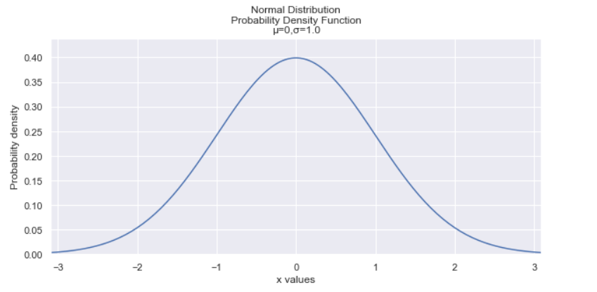
Image created by Author.
The normal distribution is arguably the most important distribution to know because many phenomena fit this distribution. IQs, heights of people, shoe size, birth weight are all examples that have a normal distribution.
The normal distribution has a bell-shaped curve and has the following properties:
- It has a symmetric bell shape.
- The mean and median are equal and are both located at the center of the distribution.
- ≈68% of the data falls within 1 standard deviation of the mean, ≈95% of the data falls within 2 standard deviations of the mean, and ≈99.7% of the data falls within 3 standard deviations of the mean.
The normal distribution is also an integral part of statistics, as it is the basis of several statistical inference techniques, including linear regression, confidence intervals, and hypothesis testing.
2. T-distribution
The t-distribution is similar to the normal distribution but is generally shorter and has fatter tails. It is used instead of the normal distribution when the sample sizes are small.
One thing to note is that as the sample size increases, the t-distribution converges to the normal distribution.
3. Gamma Distribution
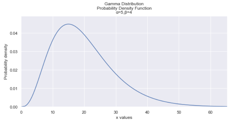
Image created by Author.
The Gamma distribution is used to predict the wait time until a future event occurs. It is useful when something has a natural minimum of 0.
It’s also generalized distribution of the chi-squared distribution and the exponential distribution (which we’ll talk about later).
4. Chi-Squared Distribution
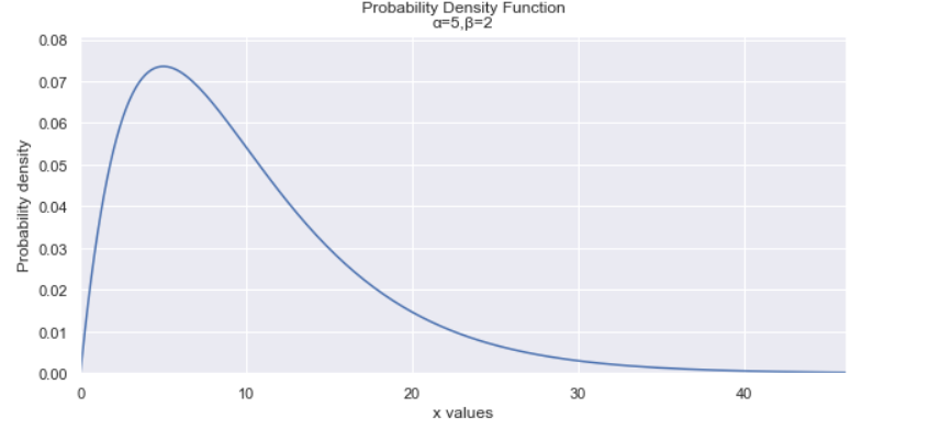
Image created by Author.
As said above, the chi-squared distribution is a particular case of the gamma distribution. As there’s a lot to the chi-squared distribution, I won’t go into too much detail, but there are several uses for it:
- It allows you to estimate confidence intervals for a population standard deviation.
- It is the distribution of sample variances when the underlying distribution is normal.
- You can test deviances of differences between expected and observed values.
- You can conduct a chi-squared test.
Note: Don’t worry so much if this one confused you because the following distributions are much simpler to understand and get a grasp of!
5. Uniform Distribution
The uniform distribution is really simple — each outcome has an equal probability. An example of this is rolling a dye.
The image above shows a distribution that is approximately uniformly distributed.
6. Bernoulli Distribution
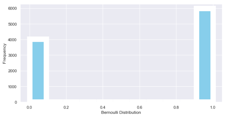
Image created by Author.
In order to understand the Bernoulli Distribution, you first need to know what a Bernoulli trial is. A Bernoulli trial is a random experiment with only two possible outcomes, success or failure, where the probability of success is the same every time.
Therefore, the Bernoulli distribution is a discrete distribution for one Bernoulli trial.
For example, flipping a coin can be represented by a Bernoulli distribution, as well as rolling an odd number on a dye.
7. Binomial Distribution
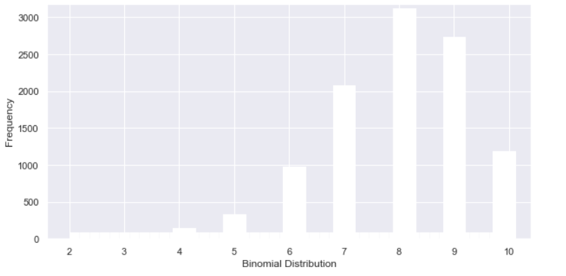
Image created by Author.
Now that you understand the Bernoulli distribution, the binomial distribution simply represents multiple Bernoulli trials. Specifically, the binomial distribution is a discrete distribution that represents the probability of getting x successes out of n independent Bernoulli trials.
Here are some examples that use the binomial distribution:
- What is the probability of getting 5 heads out of 10 coin flips?
- What is the probability of getting 10 conversions out of 100 emails (assuming the probability of converting is the same)?
- What is the probability of getting 20 responses from 500 customer feedback surveys (assuming the probability of getting a response is the same)?
One interesting thing about the binomial distribution is that it converges to a normal distribution as n (# of Bernoulli trials) gets large.
8. Geometric Distribution
The geometric distribution is also related to the Bernoulli distribution, like the binomial distribution, except that it answers a slightly different question. The geometric distribution represents the probability of having x Bernoulli (p) failures until first success? In other words, it answers, “how many trials are needed until your first success?”
An example of this is, “how many lottery tickets do I need to buy until I buy a winning ticket?”
You can also use the geometric distribution to find the probability of the number of Bernoulli (1-p) successes until failure. The geometric can also be used to check if an event is i.i.d if it fits the distribution.
9. Weibull Distribution
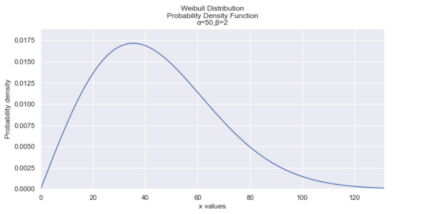
Image created by Author.
The Weibull distribution is like the geometric distribution, except it is a continuous distribution. Therefore, the Weibull distribution models the amount of time it takes for something to fail or the time between failures.
The Weibull distribution can answer questions like:
- How long until a particular lightbulb dies?
- How long until a customer churns?
10. Poisson Distribution
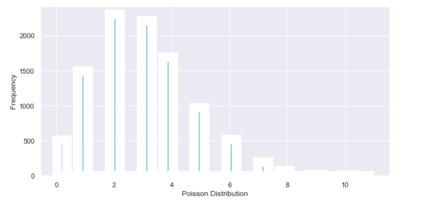
Image created by Author.
The Poisson distribution is a discrete distribution that represents how many times an event is likely to occur within a specific time period.
The Poisson distribution is most commonly used in queuing theory, which answers questions along the lines of “how many customers are likely to come (queue) within a given period of time?”.
11. Exponential Distribution
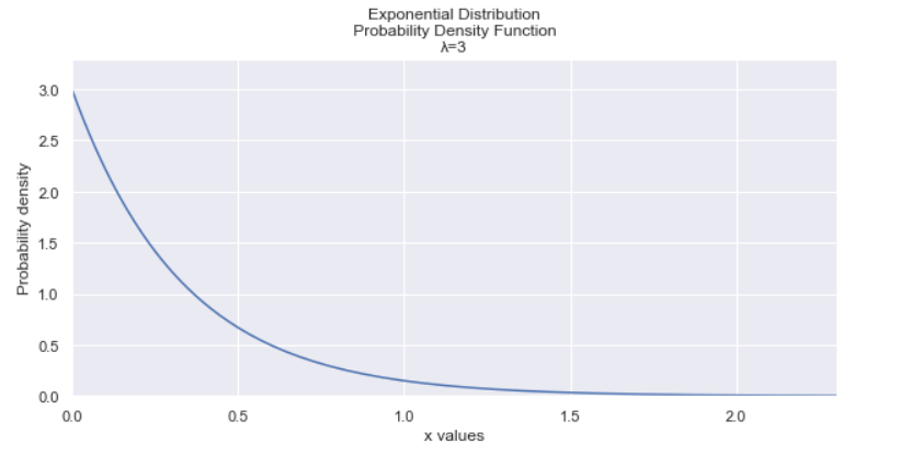
Image created by Author.
The exponential distribution is closely related to the Poisson distribution. If arrivals are distributed Poisson, then the time between arrivals (aka inter-arrival times) has the exponential distribution.
Original. Reposted with permission.
Related: