Understanding Decision Trees for Classification in Python
This tutorial covers decision trees for classification also known as classification trees, including the anatomy of classification trees, how classification trees make predictions, using scikit-learn to make classification trees, and hyperparameter tuning.
By Michael Galarnyk, Data Scientist
Decision trees are a popular supervised learning method for a variety of reasons. Benefits of decision trees include that they can be used for both regression and classification, they are easy to interpret and they don’t require feature scaling. They have several flaws including being prone to overfitting. This tutorial covers decision trees for classification also known as classification trees.
Additionally, this tutorial will cover:
- The anatomy of classification trees (depth of a tree, root nodes, decision nodes, leaf nodes/terminal nodes).
- How classification trees make predictions
- How to use scikit-learn (Python) to make classification trees
- Hyperparameter tuning
As always, the code used in this tutorial is available on my github (anatomy, predictions). With that, let’s get started!
What are Classification Trees?
Classification and Regression Trees (CART) is a term introduced by Leo Breiman to refer to the Decision Tree algorithm that can be learned for classification or regression predictive modeling problems. This post covers classification trees.
Classification Trees
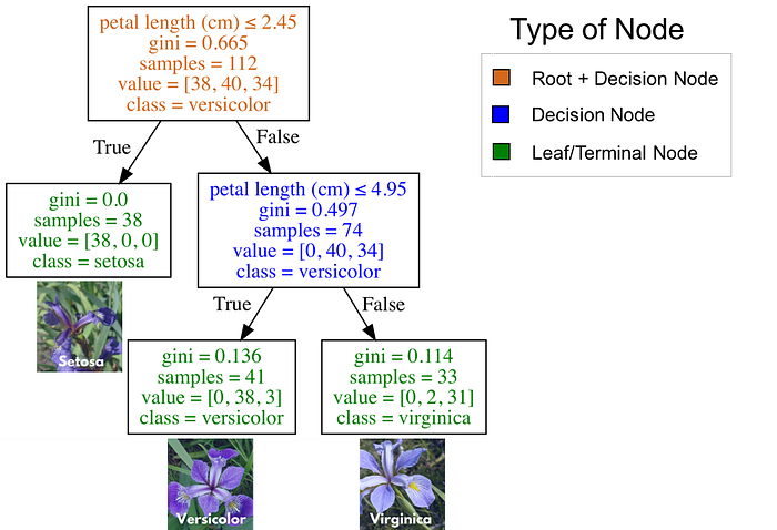
Classification trees are essentially a series of questions designed to assign a classification. The image below is a classification tree trained on the IRIS dataset (flower species). Root (brown) and decision (blue) nodes contain questions which split into subnodes. The root node is just the topmost decision node. In other words, it is where you start traversing the classification tree. The leaf nodes (green), also called terminal nodes, are nodes that don’t split into more nodes. Leaf nodes are where classes are assigned by majority vote.
How to use a Classification Tree
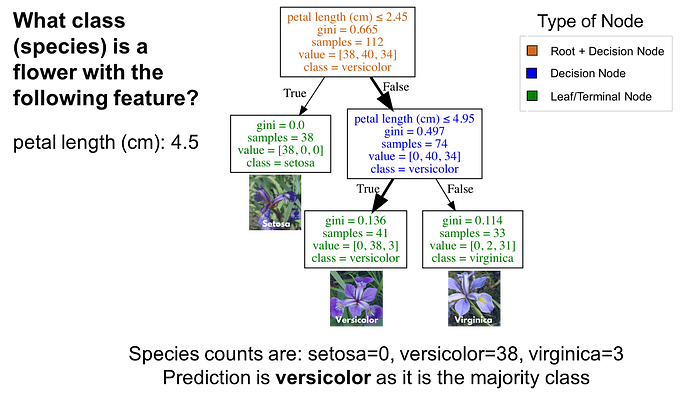
To use a classification tree, start at the root node (brown), and traverse the tree until you reach a leaf (terminal) node. Using the classification tree in the the image below, imagine you had a flower with a petal length of 4.5 cm and you wanted to classify it. Starting at the root node, you would first ask “Is the petal length (cm) ≤ 2.45”? The length is greater than 2.45 so that question is False. Proceed to the next decision node and ask, “Is the petal length (cm) ≤ 4.95”? This is True so you could predict the flower species as versicolor. This is just one example.
How are Classification Trees Grown? (Non Math Version)
A classification tree learns a sequence of if then questions with each question involving one feature and one split point. Look at the partial tree below (A), the question, “petal length (cm) ≤ 2.45” splits the data into two branches based on some value (2.45 in this case). The value between the nodes is called a split point. A good value (one that results in largest information gain) for a split point is one that does a good job of separating one class from the others. Looking at part B of the figure below, all the points to the left of the split point are classified as setosa while all the points to the right of the split point are classified as versicolor.
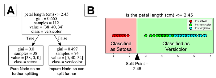
The figure shows that setosa was correctly classified for all 38 points. It is a pure node. Classification trees don’t split on pure nodes. It would result in no further information gain. However, impure nodes can split further. Notice the rightside of figure B shows that many points are misclassified as versicolor. In other words, it contains points that are of two different classes (virginica and versicolor). Classification trees are a greedy algorithm which means by default it will continue to split until it has a pure node. Again, the algorithm chooses the best split point (we will get into mathematical methods in the next section) for the impure node.
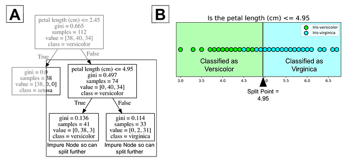
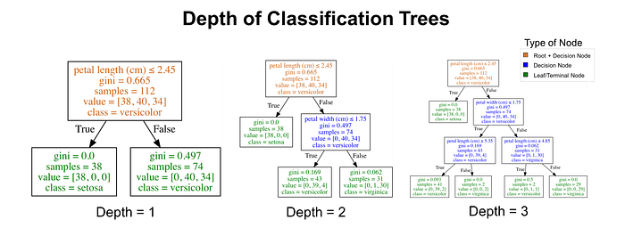
In the image above, the tree has a maximum depth of 2. Tree depth is a measure of how many splits a tree can make before coming to a prediction. This process could be continued further with more splitting until the tree is as pure as possible. The problem with many repetitions of this process is that this can lead to a very deep classification tree with many nodes. This often leads to overfitting on the training dataset. Luckily, most classification tree implementations allow you to control for the maximum depth of a tree which reduces overfitting. For example, Python’s scikit-learn allows you to preprune decision trees. In other words, you can set the maximum depth to stop the growth of the decision tree past a certain depth. For a visual understanding of maximum depth, you can look at the image below.
The Selection Criterion
This section answers how information gain and two criterion gini and entropy are calculated.
This section is really about understanding what is a good split point for root/decision nodes on classification trees. Decision trees split on the feature and corresponding split point that results in the largest information gain (IG) for a given criterion (gini or entropy in this example). Loosely, we can define information gain as
IG = information before splitting (parent) — information after splitting (children)
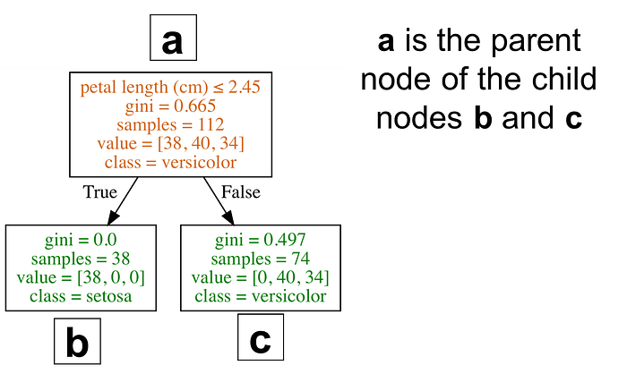
For a clearer understanding of parent and children, look at the decision tree below.
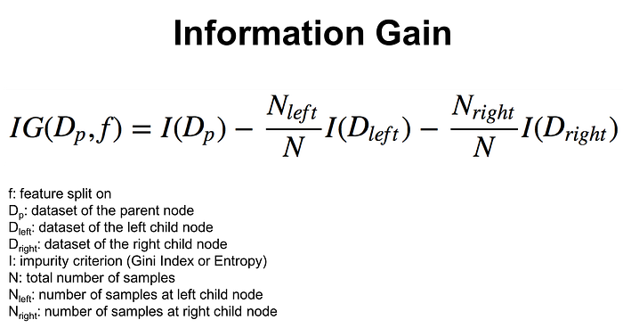
A more proper formula for information gain formula is below.
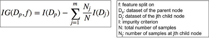
Since classification trees have binary splits, the formula can be simplified into the formula below.
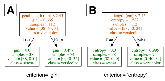
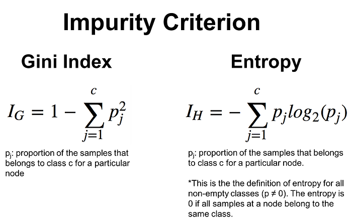
Two common criterion I, used to measure the impurity of a node are Gini index and entropy.
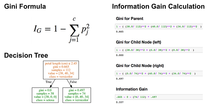
For the sake of understanding these formulas a bit better, the image below shows how information gain was calculated for a decision tree with Gini criterion.
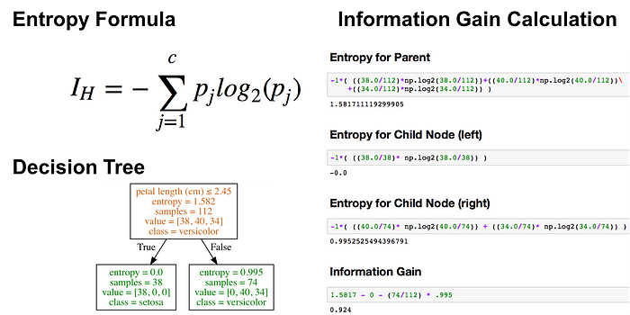
The image below shows how information gain was calculated for a decision tree with entropy.
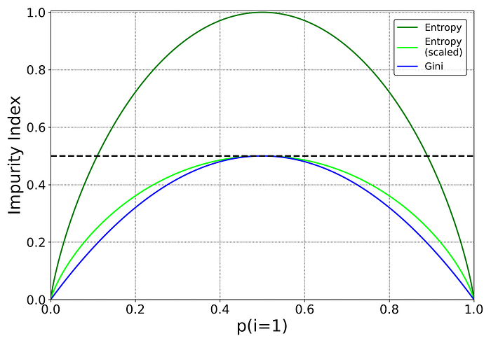
I am not going to go into more detail on this as it should be noted that different impurity measures (Gini index and entropy) usually yield similar results. The graph below shows that Gini index and entropy are very similar impurity criterion. I am guessing one of the reasons why Gini is the default value in scikit-learn is that entropy might be a little slower to compute (because it makes use of a logarithm).
Before finishing this section, I should note that are various decision tree algorithms that differ from each other. Some of the more popular algorithms are ID3, C4.5, and CART. Scikit-learn uses an optimized version of the CART algorithm. You can learn about it’s time complexity here.
Classification Trees using Python
The previous sections went over the theory of classification trees. One of the reasons why it is good to learn how to make decision trees in a programming language is that working with data can help in understanding the algorithm.
Load the Dataset
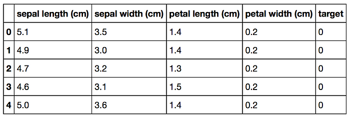
The Iris dataset is one of datasets scikit-learn comes with that do not require the downloading of any file from some external website. The code below loads the iris dataset.
import pandas as pd
from sklearn.datasets import load_irisdata = load_iris()
df = pd.DataFrame(data.data, columns=data.feature_names)
df['target'] = data.target
Splitting Data into Training and Test Sets
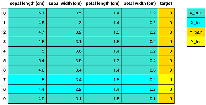
The code below puts 75% of the data into a training set and 25% of the data into a test set.
X_train, X_test, Y_train, Y_test = train_test_split(df[data.feature_names], df['target'], random_state=0)
Note, one of the benefits of Decision Trees is that you don’t have to standardize your data unlike PCA and logistic regression which are sensitive to effects of not standardizing your data.
Scikit-learn 4-Step Modeling Pattern
Step 1: Import the model you want to use
In scikit-learn, all machine learning models are implemented as Python classes
from sklearn.tree import DecisionTreeClassifier
Step 2: Make an instance of the Model
In the code below, I set the max_depth = 2 to preprune my tree to make sure it doesn’t have a depth greater than 2. I should note the next section of the tutorial will go over how to choose an optimal max_depth for your tree.
Also note that in my code below, I made random_state = 0 so that you can get the same results as me.
clf = DecisionTreeClassifier(max_depth = 2,
                             random_state = 0)
Step 3: Train the model on the data
The model is learning the relationship between X(sepal length, sepal width, petal length, and petal width) and Y(species of iris)
clf.fit(X_train, Y_train)
Step 4: Predict labels of unseen (test) data
# Predict for 1 observation
clf.predict(X_test.iloc[0].values.reshape(1, -1))# Predict for multiple observations
clf.predict(X_test[0:10])
Remember, a prediction is just the majority class of the instances in a leaf node.
Measuring Model Performance
While there are other ways of measuring model performance (precision, recall, F1 Score, ROC Curve, etc), we are going to keep this simple and use accuracy as our metric.
Accuracy is defined as:
(fraction of correct predictions): correct predictions / total number of data points
# The score method returns the accuracy of the model
score = clf.score(X_test, Y_test)
print(score)
Tuning the Depth of a Tree
Finding the optimal value formax_depth is one way way to tune your model. The code below outputs the accuracy for decision trees with different values for max_depth.
# List of values to try for max_depth:
max_depth_range = list(range(1, 6))# List to store the average RMSE for each value of max_depth:
accuracy = []for depth in max_depth_range:

    clf = DecisionTreeClassifier(max_depth = depth,
                             random_state = 0)
    clf.fit(X_train, Y_train)    score = clf.score(X_test, Y_test)
    accuracy.append(score)
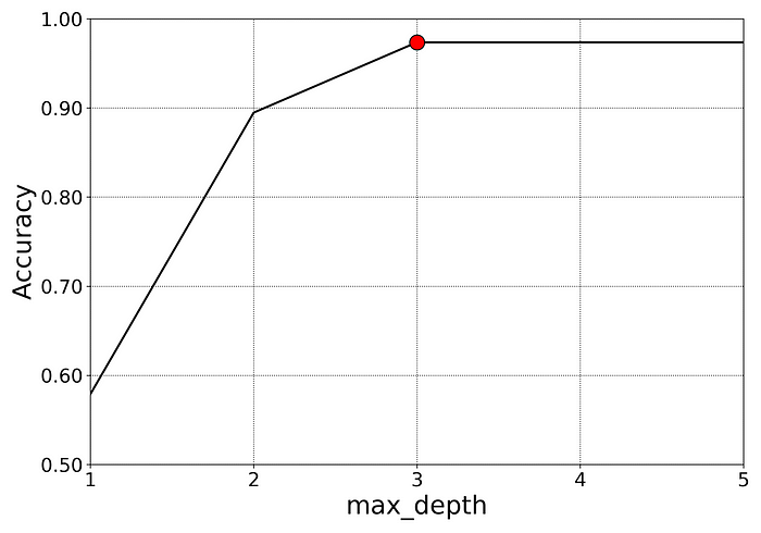
Since the graph below shows that the best accuracy for the model is when the parameter max_depth is greater than or equal to 3, it might be best to choose the least complicated model with max_depth = 3.
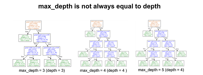
It is important to keep in mind that max_depth is not the same thing as depth of a decision tree. max_depth is a way to preprune a decision tree. In other words, if a tree is already as pure as possible at a depth, it will not continue to split. The image below shows decision trees with max_depth values of 3, 4, and 5. Notice that the trees with a max_depth of 4 and 5 are identical. They both have a depth of 4.
If you ever wonder what the depth of your trained decision tree is, you can use the get_depth method. Additionally, you can get the number of leaf nodes for a trained decision tree by using the get_n_leaves method.
While this tutorial has covered changing selection criterion (Gini index, entropy, etc) and max_depth of a tree, keep in mind that you can also tune minimum samples for a node to split (min_samples_leaf), max number of leaf nodes (max_leaf_nodes), and more.
Feature Importance
One advantage of classification trees is that they are relatively easy to interpret. Classification trees in scikit-learn allow you to calculate feature importance which is the total amount that gini index or entropy decrease due to splits over a given feature. Scikit-learn outputs a number between 0 and 1 for each feature. All feature importances are normalized to sum to 1. The code below shows feature importances for each feature in a decision tree model.
importances = pd.DataFrame({'feature':X_train.columns,'importance':np.round(clf.feature_importances_,3)})
importances = importances.sort_values('importance',ascending=False)
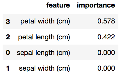
In the example above (for a particular train test split of iris), the petal width has the highest feature importance weight. We can confirm by looking at the corresponding decision tree.
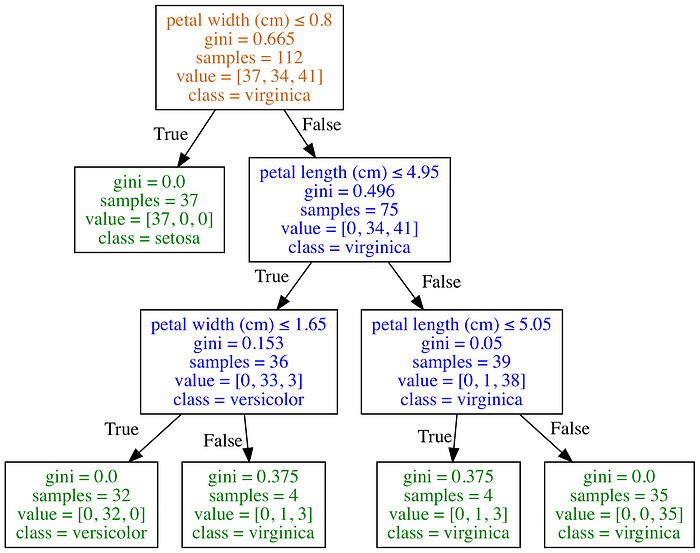
Keep in mind that if a feature has a low feature importance value, it doesn’t necessarily mean that the feature isn’t important for prediction, it just means that the particular feature wasn’t chosen at a particularly early level of the tree. It could also be that the feature could be identical or highly correlated with another informative feature. Feature importance values also don’t tell you which class they are very predictive for or relationships between features which may influence prediction. It is important to note that when performing cross validation or similar, you can use an average of the feature importance values from multiple train test splits.
Concluding Remarks
While this post only went over decision trees for classification, feel free to see my other post Decision Trees for Regression (Python). Classification and Regression Trees (CART) are a relatively old technique (1984) that is the basis for more sophisticated techniques. One of the primary weaknesses of decision trees is that they usually aren’t the most accurate algorithm. This is partially because decision trees are a high variance algorithm, meaning that different splits in the training data can lead to very different trees. If you have any questions or thoughts on the tutorial, feel free to reach out in the comments below or through Twitter.
Bio: Michael Galarnyk is a Data Scientist and Corporate Trainer. He currently works at Scripps Translational Research Institute. You can find him on Twitter (https://twitter.com/GalarnykMichael), Medium (https://medium.com/@GalarnykMichael), and GitHub (https://github.com/mGalarnyk).
Original. Reposted with permission.
Related:
- Decision Trees — An Intuitive Introduction
- How to Build a Data Science Portfolio
- Random Forests vs Neural Networks: Which is Better, and When?