5 Great New Features in Latest Scikit-learn Release

The latest release of Python's workhorse machine learning library includes a number of new features and bug fixes. You can find a full accounting of these changes from the official Scikit-learn 0.22 release highlights, and can read find the change log here.

Updating your installation is done via pip:

   pip install --upgrade scikit-learn

or conda:

   conda install scikit-learn

Here are 5 new features in the latest release of Scikit-learn which are worth your attention.

1. New Plotting API

 
A new plotting API is available, working without requiring any recomputation. Supported plots include, among others, partial dependence plots, confusion matrix, and ROC curves. Here's a demonstration of the API, using an example from Scikit-learn's user guide:

from sklearn.model_selection import train_test_split
from sklearn.svm import SVC
from sklearn.metrics import plot_roc_curve
from sklearn.datasets import load_wine

X_train, X_test, y_train, y_test = train_test_split(X, y, random_state=42)
svc = SVC(random_state=42)
svc.fit(X_train, y_train)

svc_disp = plot_roc_curve(svc, X_test, y_test)

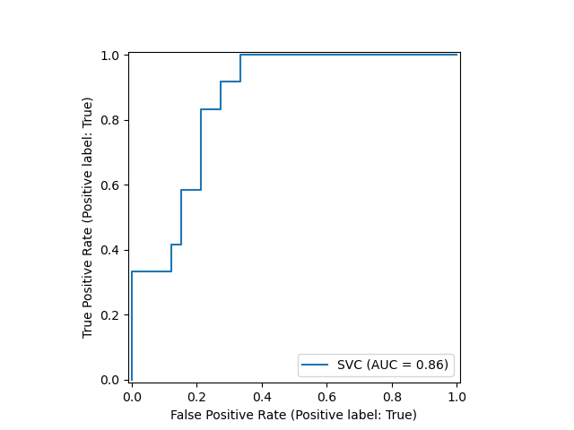
Note the plotting is done via the single last line of code.

2. Stacked Generalization

 
The ensemble learning technique of stacking estimators for bias reduction has come to Scikit-learn. StackingClassifier and StackingRegressor are the modules enabling estimator stacking, and the final_estimator uses these stacked estimator predictions as its input. See this example from the user guide, using the regression estimators defined below as estimators, with a gradient boosting regressor final estimator:

from sklearn.linear_model import RidgeCV, LassoCV
from sklearn.svm import SVR
from sklearn.ensemble import GradientBoostingRegressor
from sklearn.ensemble import StackingRegressor
from sklearn.datasets import load_boston
from sklearn.model_selection import train_test_split

estimators = [('ridge', RidgeCV()),
              ('lasso', LassoCV(random_state=42)),
              ('svr', SVR(C=1, gamma=1e-6))]

reg = StackingRegressor(
        estimators=estimators,
        final_estimator=GradientBoostingRegressor(random_state=42))

X, y = load_boston(return_X_y=True)
X_train, X_test, y_train, y_test = train_test_split(X, y, random_state=42)

reg.fit(X_train, y_train)

   StackingRegressor(...)

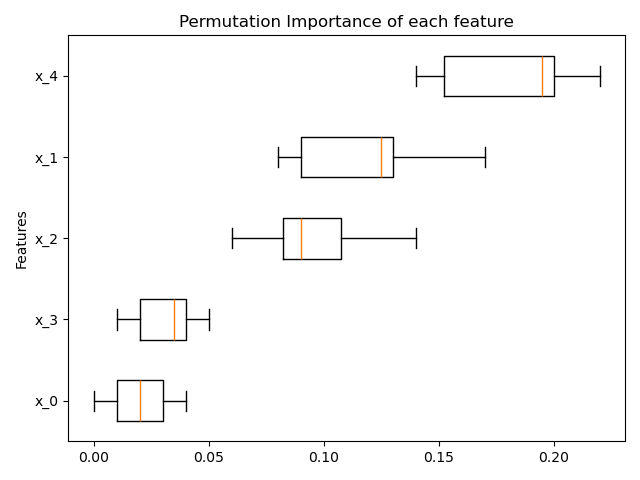
3. Feature Importance for Any Estimator

 
Permutation based feature importance is now available for any fitted Scikit-learn estimator. A description of how the permutation importance of a feature is calculated, from the user guide:

The permutation importance of a feature is calculated as follows. First, a baseline metric, defined by scoring, is evaluated on a (potentially different) dataset defined by the X. Next, a feature column from the validation set is permuted and the metric is evaluated again. The permutation importance is defined to be the difference between the baseline metric and metric from permutating the feature column.

A full example from the release notes:

from sklearn.ensemble import RandomForestClassifier
from sklearn.inspection import permutation_importance

X, y = make_classification(random_state=0, n_features=5, n_informative=3)

rf = RandomForestClassifier(random_state=0).fit(X, y)
result = permutation_importance(rf, X, y, n_repeats=10, random_state=0, n_jobs=-1)

fig, ax = plt.subplots()
sorted_idx = result.importances_mean.argsort()
ax.boxplot(result.importances[sorted_idx].T, vert=False, labels=range(X.shape[1]))
ax.set_title("Permutation Importance of each feature")
ax.set_ylabel("Features")
fig.tight_layout()
plt.show()

4. Gradient Boosting Missing Value Support

 
The gradient boosting classifier and regressor are now both natively equipped to deal with missing values, thus eliminating the need to manually impute. Here's how missing value decisions are made:

During training, the tree grower learns at each split point whether samples with missing values should go to the left or right child, based on the potential gain. When predicting, samples with missing values are assigned to the left or right child consequently. If no missing values were encountered for a given feature during training, then samples with missing values are mapped to whichever child has the most samples.

The following example demonstrates:

from sklearn.experimental import enable_hist_gradient_boosting  # noqa
from sklearn.ensemble import HistGradientBoostingClassifier
import numpy as np

X = np.array([0, 1, 2, np.nan]).reshape(-1, 1)
y = [0, 0, 1, 1]

gbdt = HistGradientBoostingClassifier(min_samples_leaf=1).fit(X, y)
print(gbdt.predict(X))

   [0 0 1 1]

5. KNN Based Missing Value Imputation

 
While gradient boosting now natively supports missing value imputation, explicit imputation can be performed on any dataset using the K-nearest neighbors imputer. Each missing value is imputed from the mean of n nearest neighbors, in the training set, so long as the features which neither sample are missing are near. Euclidean distance is the distance default metric used.

An example:

import numpy as np
from sklearn.impute import KNNImputer

X = [[1, 2, np.nan], [3, 4, 3], [np.nan, 6, 5], [8, 8, 7]]
imputer = KNNImputer(n_neighbors=2)
print(imputer.fit_transform(X))

[[1.  2.  4. ]
 [3.  4.  3. ]
 [5.5 6.  5. ]
 [8.  8.  7. ]]

There are more features in the latest release of Scikit-learn which were not covered here. You may want to check out the full release highlights and change log for more information.

Happy machine learning!

 
Related:

• Train sklearn 100x Faster
• How to Extend Scikit-learn and Bring Sanity to Your Machine Learning Workflow
• Scikit-Learn & More for Synthetic Dataset Generation for Machine Learning