Explainability: Cracking open the black box, Part 1
What is Explainability in AI and how can we leverage different techniques to open the black box of AI and peek inside? This practical guide offers a review and critique of the various techniques of interpretability.
By Manu Joseph, Problem Solver, Practitioner, Researcher at Thoucentric Analytics.

Interpretability is the degree to which a human can understand the cause of a decision – Miller, Tim
Explainable AI (XAI) is a sub-field of AI which has been gaining ground in the recent past. And as I machine learning practitioner dealing with customers day in and day out, I can see why. I’ve been an analytics practitioner for more than 5 years, and I swear, the hardest part of a machine learning project is not creating the perfect model which beats all the benchmarks. It’s the part where you convince the customer why and how it works.

Evolution of papers about XAI in the last few years from Arrieta, et al.
Humans always had a dichotomy when faced with the unknown. Some of us deal with it using faith and worship it, like our ancestors who worshipped fire, the skies, etc. And some of us turn to distrust. Likewise, in Machine Learning, there are people who are satisfied by rigorous testing of the model (i.e., the performance of the model) and those who want to know why and how a model is doing what it is doing. And there is no right or wrong here.
Yann LeCun, Turing Award winner and Facebook’s Chief AI Scientist and Cassie Kozyrkov, Google’s Chief Decision Intelligence Engineer, are strong proponents of the line of thought that you can infer a model’s reasoning by observing its actions (i.e., predictions in a supervised learning framework). On the other hand Microsoft Research’s Rich Caruana and a few others have insisted that the models inherently have interpretability and not just derived through the performance of the model.
We can spend years debating the topic, but for the widespread adoption of AI, explainable AI is essential and is increasingly demanded from the industry. So, here I am attempting to explain and demonstrate a few interpretability techniques which have been useful for me in both explaining the model to a customer, as well as investigating a model and make it more reliable.
What is Interpretability?
Interpretability is the degree to which a human can understand the cause of a decision. And in the artificial intelligence domain, it means it is the degree to which a person can understand the how and why of an algorithm and its predictions. There are two major ways of looking at this – Transparency and Post-hoc Interpretation.
TRANSPARENCY
Transparency addresses how well the model can be understood. This is inherently specific to the model that we use.
One of the key aspects of such transparency is simulatability. Simulatability denotes the ability of a model of being simulated or thought about strictly by a human[3]. Complexity of the model plays a big part in defining this characteristic. While a simple linear model or a single layer perceptron is simple enough to think about, it becomes increasingly difficult to think about a decision tree with a depth of, say, 5. It also becomes harder to think about a model that has a lot of features. Therefore it follows that a sparse linear model(Regularized Linear Model) is more interpretable than a dense one.
Decomposability is another major tenet of transparency. It stands for the ability to explain each of the parts of a model (input, parameter, and calculation)[3]. It requires everything from input(no complex features) to output to be explained without the need for another tool.
The third tenet of transparency is Algorithmic Transparency. This deals with the inherent simplicity of the algorithm. It deals with the ability of a human to fully understand the process an algorithm takes to convert inputs to an output.
POST-HOC INTERPRETATION
Post-hoc interpretation is useful when the model itself is not transparent. So in the absence of clarity on how the model is working, we resort to explaining the model and its predictions using a multitude of ways. Arrieta, Alejandro Barredo et al. have compiled and categorized them into 6 major buckets. We will be talking about some of these here.
- Visual Explanations – These sets of methods try to visualize the model behaviour to try and explain them. The majority of the techniques that fall in this category uses techniques like dimensionality reduction to visualize the model in a human-understandable format.
- Feature Relevance Explanations – These sets of methods try to expose the inner workings of a model by computing feature relevance or importance. These are thought of as an indirect way of explaining a model.
- Explanations by simplification – These sets of methods try to train the whole new system based on the original model to provide explanations.
Since this a wide topic and covering all of it would be a humongous blog post, I’ve split it into multiple parts. We will cover the interpretable models and the ‘gotchas’ in it in the current part and leave the post-hoc analysis for the next one.
Interpretable Models
Occam’s Razor states that simple solutions are more likely to be correct than complex ones. In data science, Occam’s Razor is usually stated in conjunction with overfitting. But I believe it is equally applicable in the explainability context. If you can get the performance that you desire with a transparent model, look no further in your search for the perfect algorithm.
Arrieta, Alejandro Barredo et al. have summarised the ML models and categorised them in a nice table.

LINEAR/LOGISTIC REGRESSION
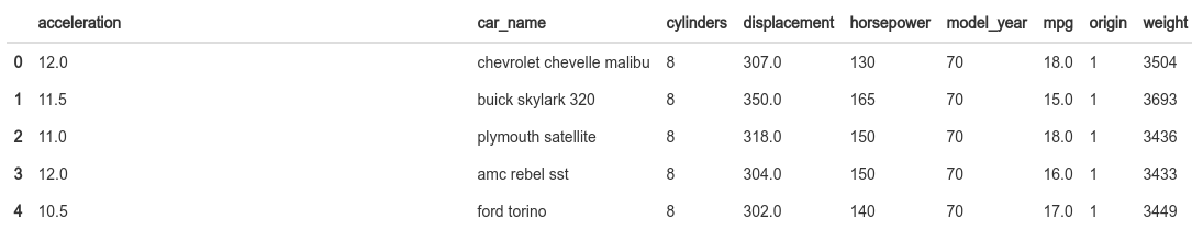
Since Logistic Regression is also a linear regression in some way, we just focus on Linear Regression. Let’s take a small data set (auto-mpg) to investigate the model. The data concerns city-cycle fuel consumption in miles per gallon along with different attributes of the car like:
- cylinders: multi-valued discrete
- displacement: continuous
- horsepower: continuous
- weight: continuous
- acceleration: continuous
- model year: multi-valued discrete
- origin: multi-valued discrete
- car name: string (unique for each instance)
After loading the data, the first step is to run pandas_profiling.
import pandas as pd

import numpy as np

import pandas_profiling

import pathlib

import cufflinks as cf

#We set the all charts as public

cf.set_config_file(sharing='public',theme='pearl',offline=False)

cf.go_offline()

cwd = pathlib.Path.cwd()

data = pd.read_csv(cwd/'mpg_dataset'/'auto-mpg.csv')

report = data.profile_report()

report.to_file(output_file="auto-mpg.html")
Just one line of code and this brilliant library does your preliminary EDA for you.

Snapshot from the Pandas Profiling Report. Click here to view the full report.
DATA PREPROCESSING
- Right off the bat, we see that car nameshave 305 distinct values in 396 rows. So we drop that variable.
- horsepoweris interpreted as a categorical variable. Upon investigation, it had some rows with “?”. Replaced them with the mean of the column and converted it to float.
- It also shows multicollinearity between displacement, cylinders, and weight. Let’s leave it in there for now.
In the python world, Linear regression is available in Sci-kit Learn and Statsmodels. Both of them give the same results, but Statsmodels is more leaning towards statisticians and Sci-kit Learn towards ML practitioners. Let’s use statsmodels because of the beautiful summary it provides out of the box.
X = data.drop(['mpg'], axis=1)

y = data['mpg']

## let's add an intercept (beta_0) to our model

# Statsmodels does not do that by default

X = sm.add_constant(X)

model = sm.OLS(y, X).fit()

predictions = model.predict(X)


# Print out the statistics

model.summary()

# Plot the coefficients (except intercept)

model.params[1:].iplot(kind='bar')


The interpretation is really straightforward here.
- Intercept can be interpreted as the mileage you would predict for a case where all the independent variables are zero. The ‘gotcha’ here is that, if it is not reasonable that the independent variables can be zero or if there are no such occurrences in the data on which the Linear Regression was trained, then the intercept is quite meaningless. It just anchors the regression in the right place.
- The coefficients can be interpreted as the change in the dependent variable which would drive a unit change in independent variable. For example, if we increase the weight by 1, the mileage would drop by 0.0067
- Some features like cylinders, model year, etc, are categorical in nature. Such coefficients need to be interpreted as the average difference in mileage between the different categories. One more caveat here is that all the categorical features are also ordinal(more cylinders means less mileage, or higher the model_year better the mileage) in nature, and hence it’s OK to just leave them as is and run the regression. But if that is not the case, dummy or one-hot encoding the categorical variables is the way to go.
Now coming to the feature importance, looks like origin, and model year are the major features that drive the model, right?
Nope. Let’s look at it in detail. To make my point clear, let’s look at a few rows of the data.
origin has values like 1, 2, etc., model_year has values like 70,80, etc., weight has values like 3504, 3449 etc., and mpg(our dependent variable) has values like 15,16,etc. You see the problem here? To make an equation which outputs 15 or 16, the equation needs to have a small coefficient for weight, and a large coefficient for origin.
So, what do we do?
Enter, Standardized Regression Coefficients.

We multiply each of the coefficients with the ratio of standard deviation of the independent variable to standard deviation of the dependent variable. Standardized coefficients refer to how many standard deviations a dependent variable will change, per standard deviation increase in the predictor variable.
#Standardizing the Regression coefficients

std_coeff = model.params

for col in X.columns:

std_coeff[col] = (std_coeff[col]* np.std(X[col]))/ np.std(y)

std_coeff[1:].round(4).iplot(kind='bar')

The picture really changed, didn’t it? The weight of the car, whose coefficient was almost zero, turned out to be the biggest driver in determining mileage. If you want to get more intuition/math behind the standardization, I suggest you check out this stackoverflow answer.
Another way you can get similar results is by standardizing the input variables before fitting the linear regression and then examining the coefficients.
from sklearn.preprocessing import StandardScaler

scaler = StandardScaler()

X_std = scaler.fit_transform(X)

lm = LinearRegression()

lm.fit(X_std,y)

r2 = lm.score(X_std,y)

adj_r2 = 1-(1-r2)*(len(X)-1)/(len(X)-len(X.columns)-1)

print ("R2 Score: {:.2f}% | Adj R2 Score: {:.2f}%".format(r2*100,adj_r2*100))

params = pd.Series({'const': lm.intercept_})

for i,col in enumerate(X.columns):

params[col] = lm.coef_[i]

params[1:].round(4).iplot(kind='bar')

Even though the actual coefficients are different, the relative importance between the features remains the same.
The final ‘gotcha’ in Linear Regression is around multicollinearity and OLS in general. Linear Regression is solved using OLS, which is an unbiased estimator. Even though it sounds like a good thing, it is not necessarily. What ‘unbiased’ here means is that the solving procedure doesn’t consider which independent variable is more important than the others; i.e., it is unbiased towards the independent variables and strives to achieve the coefficients which minimize the Residual Sum of Squares. But do we really want a model that just minimizes the RSS? Hint: RSS is computed in the training set.
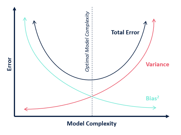
In the Bias vs Variance tradeoff, there exists a sweet spot where you get optimal model complexity, which avoids overfitting. And usually since it is quite difficult to estimate bias and variance to do analytical reasoning and arrive at the optimal point, we employ cross-validation based strategies to achieve the same. But, if you think about it, there is no real hyperparameter to tweak in a Linear Regression.
And, since the estimator is unbiased, it will allocate a fraction of contribution to every feature available to it. This becomes more of a problem when there is multicollinearity. While this doesn’t affect the predictive power of the model much, it does affect the interpretability of it. When one feature is highly correlated with another feature or a combination of features, the marginal contribution of that feature is influenced by the other features. So, if there is strong multi-collinearity in your dataset, the regression coefficients will be misleading.
Enter Regularization.
At the heart of almost any machine learning algorithm is an optimization problem that minimizes a cost function. In the case of Linear Regression, that cost function is Residual Sum of Squares, which is nothing but the squared error between the prediction and the ground truth parametrized by the coefficients.

Source: https://web.stanford.edu/~hastie/ElemStatLearn/
To add regularization, we introduce an additional term to the cost function of the optimization. The cost function now becomes:

Ridge Regression (L2 Regularization)

Lasso Regression (L1 regularization)
In Ridge Regression we added the sum of all squared coefficients to the cost function, and in Lasso Regression we added the sum of absolute coefficients. In addition to those, we also introduced a parameter which is a hyperparameter we can tune to arrive at the optimum model complexity. And by virtue of the mathematical properties of L1 and L2 regularization, the effect on the coefficients are slightly different.
- Ridge Regression shrinks the coefficients to near zero for the independent variables it deems less important.
- Lasso Regression shrinks the coefficients to zero for the independent variables it deems less important.
- If there is multicollinearity, Lasso selects one of them and shrinks the other to zero, whereas Ridge shrinks the other one to near zero.
Elements of Statistical Learning by Hastie, Tibshirani, Friedman gives the following guideline: When you have many small/medium sized effects you should go with Ridge. If you have only a few variables with a medium/large effect, go with Lasso. You can check out this medium blog which explains Regularization in quite detail. The author has also given a succinct summary which I’m borrowing here.

lm = RidgeCV()

lm.fit(X,y)

r2 = lm.score(X,y)

adj_r2 = 1-(1-r2)*(len(X)-1)/(len(X)-len(X.columns)-1)

print ("R2 Score: {:.2f}% | Adj R2 Score: {:.2f}%".format(r2*100,adj_r2*100))

params = pd.Series({'const': lm.intercept_})

for i,col in enumerate(X.columns):

params[col] = lm.coef_[i]

ridge_params = params.copy()


lm = LassoCV()

lm.fit(X,y)

r2 = lm.score(X,y)

adj_r2 = 1-(1-r2)*(len(X)-1)/(len(X)-len(X.columns)-1)

print ("R2 Score: {:.2f}% | Adj R2 Score: {:.2f}%".format(r2*100,adj_r2*100))

params = pd.Series({'const': lm.intercept_})

for i,col in enumerate(X.columns):

params[col] = lm.coef_[i]

lasso_params = params.copy()

ridge_params.to_frame().join(lasso_params.to_frame(), lsuffix='_ridge', rsuffix='_lasso')
We just ran Ridge and Lasso Regression on the same data. Ridge Regression gave the exact same R2 and Adjusted R2 scores as the original regression(82.08% and 81.72%, respectively), but with slightly shrunk coefficients. And Lasso gave a lower R2 and Adjusted R2 score(76.67% and 76.19%, respectively) with considerable shrinkage.

If you look at the coefficients carefully, you can see that Ridge Regression did not shrink the coefficients much. The only place where it really shrunk is for displacement and origin. There may be two reasons for this:
- Displacement had a strong correlation with cylinders (0.95), and hence it was shrunk
- Most of the coefficients in the original problem were already close to zero and hence very little shrinkage.
But if you look at how Lasso has shrunk the coefficients, you’ll see it is quite aggressive.
- It has completely shrunk cylinders, acceleration, and origin to zero. Cylinders because of multicollinearity, acceleration because of its lack of predictive power(p-value in original regression was 0.287).
As a rule of thumb, I would suggest to always use some kind of regularization.
DECISION TREES
Let’s pick another dataset for this exercise – the world-famous Iris dataset. For those who have been living under a rock, the Iris dataset is a dataset of measurements taken for three species of flowers. One flower species is linearly separable from the other two, but the other two are not linearly separable from each other.
The columns in this dataset are:
- Id
- SepalLengthCm
- SepalWidthCm
- PetalLengthCm
- PetalWidthCm
- Species
We dropped the ‘Id’ column, encoded the Species target to make it the target, and trained a Decision Tree Classifier on it.
Let’s take a look at the “feature importance“ (we will go in detail about the feature importance and it’s interpretation in the next part of the blog series) from the Decision Tree.
clf = DecisionTreeClassifier(min_samples_split = 4)

clf.fit(X,y)

feat_imp = pd.DataFrame({'features': X.columns.tolist(), "mean_decrease_impurity": clf.feature_importances_}).sort_values('mean_decrease_impurity', ascending=False)

feat_imp = feat_imp.head(25)

feat_imp.iplot(kind='bar',

y='mean_decrease_impurity',

x='features',

yTitle='Mean Decrease Impurity',

xTitle='Features',

title='Mean Decrease Impurity',

)

Out of the four features, the classifier only used PetalLength and Petal Width to separate the three classes.
Let’s visualize the Decision Tree using the brilliant library dtreeviz and see how the model has learned the rules.
from dtreeviz.trees import *

viz = dtreeviz(clf,
X,
y,
target_name='Species',
class_names=["setosa", "versicolor", "virginica"],

feature_names=X.columns)

viz

It’s very clear how the model is doing what it is doing. Let’s go a step ahead and visualize how a particular prediction is made.
# random sample from training

x = X.iloc[np.random.randint(0, len(X)),:]

viz = dtreeviz(clf,

X,

y,

target_name='Species',

class_names=["setosa", "versicolor", "virginica"],

feature_names=X.columns,

X=x)

viz

If we rerun the classification with just the two features which the Decision Tree selected, it will give you the same prediction. But the same cannot be said of an algorithm like Linear Regression. If we remove the variables which don’t meet the p-value cutoff, the performance of the model may also go down by some amount.
Interpreting a Decision tree is a lot more straightforward than a Linear Regression, with all its quirks and assumptions. Statistical Modelling: The Two Cultures by Leo Breiman is a must-read to understand the problems in interpreting Linear Regression, and it also argues a case for Decision Trees or even Random Forests over Linear Regression, both in terms of performance and interpretability. (Disclaimer: If it has not struck you already, Leo Breiman co-invented Random Forest)
Full Code is available in my Github.
Original. Reposted with permission.
Bio: Manu Joseph (@manujosephv) is an inherently curious and self-taught Data Scientist with about 8+ years of professional experience working with Fortune 500 companies, including a researcher at Thoucentric Analytics.
Related: