Interpretability part 3: opening the black box with LIME and SHAP

By Manu Joseph, Problem Solver, Practitioner, Researcher at Thoucentric Analytics.

Previously, we looked at the pitfalls with the default “feature importance” in tree-based models, talked about permutation importance, LOOC importance, and Partial Dependence Plots. Now let’s switch lanes and look at a few model agnostic techniques which take a bottom-up way of explaining predictions. Instead of looking at the model and trying to come up with global explanations like feature importance, these sets of methods look at every single prediction and then try to explain them.

5) Local Interpretable Model-agnostic Explanations (LIME)

As the name suggests, this is a model agnostic technique to generate local explanations to the model. The core idea behind the technique is quite intuitive. Suppose we have a complex classifier, with a highly non-linear decision boundary. But if we zoom in and look at a single prediction, the behaviour of the model in that locality can be explained by a simple interpretable model (mostly linear).

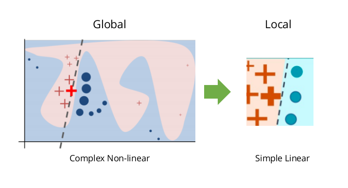
LIME localises a problem and explains the model at that locality, rather than generating an explanation for the whole model.

LIME[2] uses a local surrogate model trained on perturbations of the data point we are investigating for explanations. This ensures that even though the explanation does not have global fidelity (faithfulness to the original model) it has local fidelity. The paper[2] also recognizes that there is an interpretability vs fidelity trade-off and proposed a formal framework to express the framework.

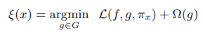
 is the explanation,  is the inverse of local fidelity (or how unfaithful is g in approximating f in the locality), and  is the complexity of the local model, g. In order to ensure both local fidelity and interpretability, we need to minimize the unfaithfulness (or maximize the local fidelity), keeping in mind that the complexity should be low enough for humans to understand.

Even though we can use any interpretable model as the local surrogate, the paper uses a Lasso regression to induce sparsity in explanations. The authors of the paper have restricted their explorations to the fidelity of the model and kept the complexity as user input. In the case of a Lasso Regression, it is the number of features for which the explanation should be attributed.

One additional aspect they have explored and proposed a solution (one which has not got a lot of popularity) is the challenge of providing a global explanation using a set of individual instances. They call it “Submodular Pick for Explaining Models.” It is essentially a greedy optimization that tries to pick a few instances from the whole lot which maximizes something they call “non-redundant coverage.” Non-redundant coverage makes sure that the optimization is not picking instances with similar explanations.

The advantages of the technique are:

• Both the methodology and the explanations are very intuitive to explain to a human being.
• The explanations generated are sparse, and thereby increasing interpretability.
• Model-agnostic
• LIME works for structured as well as unstructured data(text, images)
• Readily available in R and Python (original implementation by the authors of the paper)
• Ability to use other interpretable features even when the model is trained in complex features like embeddings and the likes. For example, a regression model may be trained on a few components of a PCA, but the explanations can be generated on original features which makes sense to a human.

ALGORITHM

• To find an explanation for a single data point and a given classifier
• Sample the locality around the selected single data point uniformly and at random and generate a dataset of perturbed data points with its corresponding prediction from the model we want to be explained
• Use the specified feature selection methodology to select the number of features that is required for explanation
• Calculate the sample weights using a kernel function and a distance function. (this captures how close or how far the sampled points are from the original point)
• Fit an interpretable model on the perturbed dataset using the sample weights to weigh the objective function.
• Provide local explanations using the newly trained interpretable model

IMPLEMENTATION

The implementation by the paper authors is available in Github as well as a installable package in pip. Before we take a look at how we would implement those, let’s discuss a few quirks in the implementation which you should know before running with it (focus on tabular explainer).

The main steps are as follows

• Initialize a TabularExplainer by providing the data in which it was trained (or the training data stats if training data is not available), some details about the features and class names(in case of classification)
• Call a method in the class, explain_instance, and provide the instance for which you need an explanation, the predict method of your trained model, and the number of features you need to include in the explanation.

The key things you need to keep in mind are:

• By default modeis classification. So if you are trying to explain a regression problem, be sure to mention it.
• By default, the feature selection is set to ‘auto.’ ‘auto’ chooses between forward selection and highest weights based on the number of features in the training data (if it is less than 6, forward selection). The highest weights just fit a Ridge Regression on the scaled data and selects the n highest weights. If you specify ‘none’ as the feature selection parameter, it does not do any feature selection. And if you pass ‘lasso_path’ as the feature selection, it uses lasso_path from sklearn to find the right level regularization which provides n non-zero features.
• By default, Ridge Regression is used as the interpretable model. But you can pass in any sci-kit learn model you want as long as it has coef_ and ‘sample_weight’ as parameters.
• There are two other key parameters, kernel and kernel_width, which determines the way the sample weights are calculated and also limits the locality in which perturbation can happen. These are kept as a hyperparameter in the algorithm. Although, in most use cases, the default values would work.
• By default, discretize_continuousis set to True. This means that the continuous features are discretized to either quartiles, deciles, or based on Entropy. The default value for discretizer is quartile.

Now, let’s continue with the same dataset we have been working with in the last part and see LIME in action.

import lime
import lime.lime_tabular
 
# Creating the Lime Explainer
# Be very careful in setting the order of the class names
lime_explainer = lime.lime_tabular.LimeTabularExplainer(
    X_train.values,
    training_labels=y_train.values,
    feature_names=X_train.columns.tolist(),
    feature_selection="lasso_path",
    class_names=["<50k", ">50k"],
    discretize_continuous=True,
    discretizer="entropy",
)
#Now let's pick a sample case from our test set.
row = 345

Row 345.

exp = lime_explainer.explain_instance(X_test.iloc[row], rf.predict_proba, num_features=5)
 
exp.show_in_notebook(show_table=True)

For variety, let’s look at another example. One which the model mis-classified.

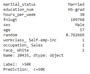
Row 26.

INTERPRETATION

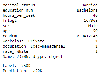
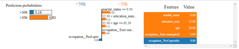
Example 1

• The first example we looked at is a 50-year-old married man with a Bachelors's degree. He is working in a private firm in an executive/managerial position for 40 hours every week. Our model has rightly classified him as earning above 50k
• The prediction as such makes sense in our mental model. Somebody who is 50 years old and working in a managerial position has a very high likelihood of earning more than 50k.
• If we look at how the model has made that decision, we can see that it is attributed to his marital status, age, education and the fact that he is in an executive/managerial role. The fact that his occupation is not a professional-specialty has tried to pull down his likelihood, but overall the model has decided that it is highly likely that this person earns above 50k

Example 2

• The second example we have is a 57-year-old, married man with a High School Degree. He is a self-employed person working in sales and he just works 30 hours a week.
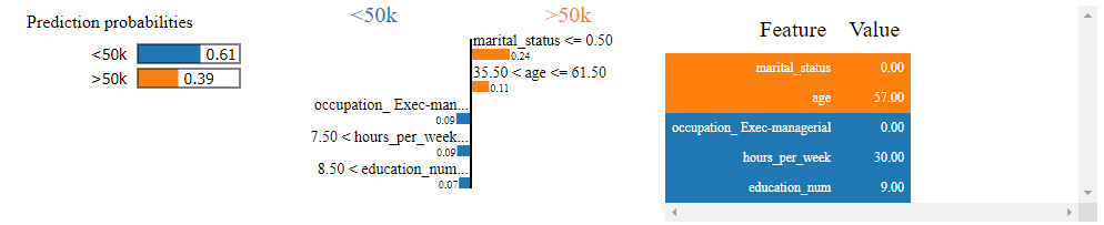
• Even in our mental model, it is slightly difficult for us to predict whether such a person is earning more than 50k or not. And the model went ahead and predicted that this person is earning less than 50k, where in fact he is earning more.
• If we look at how the model has made this decision, we can see that there is a strong push and pull effect in the locality of the prediction. On one side his marital_status and age are working to push him towards the above 50k bucket. And on the other side, the fact that he is not an executive/manager, his education, and hours per week is working towards pushing him down. And in the end, the downward push won the game and the model predicted his income to be below 50k.

SUBMODULAR PICK AND GLOBAL EXPLANATIONS

As mentioned earlier, there is another technique mentioned in the paper called “submodular pick” to find a handful of explanations which try to explain most of the cases. Let’s try to get that as well. This particular part of the python library is not so stable and the example notebooks provided was giving me errors. But after spending sometime reading through the source code, I figured out a way out of the errors.

from lime import submodular_pick
sp_obj = submodular_pick.SubmodularPick(lime_explainer, X_train.values, rf.predict_proba, sample_size=500, num_features=10, num_exps_desired=5)
#Plot the 5 explanations
[exp.as_pyplot_figure(label=exp.available_labels()[0]) for exp in sp_obj.sp_explanations];
# Make it into a dataframe
W_pick=pd.DataFrame([dict(this.as_list(this.available_labels()[0])) for this in sp_obj.sp_explanations]).fillna(0)
 
W_pick['prediction'] = [this.available_labels()[0] for this in sp_obj.sp_explanations]
 
#Making a dataframe of all the explanations of sampled points
W=pd.DataFrame([dict(this.as_list(this.available_labels()[0])) for this in sp_obj.explanations]).fillna(0)
W['prediction'] = [this.available_labels()[0] for this in sp_obj.explanations]
 
#Plotting the aggregate importances
np.abs(W.drop("prediction", axis=1)).mean(axis=0).sort_values(ascending=False).head(
    25
).sort_values(ascending=True).iplot(kind="barh")
 
#Aggregate importances split by classes
grped_coeff = W.groupby("prediction").mean()
 
grped_coeff = grped_coeff.T
grped_coeff["abs"] = np.abs(grped_coeff.iloc[:, 0])
grped_coeff.sort_values("abs", inplace=True, ascending=False)
grped_coeff.head(25).sort_values("abs", ascending=True).drop("abs", axis=1).iplot(
    kind="barh", bargap=0.5
) 

Click for full interactive plot

Click for full interactive plot

INTERPRETATION

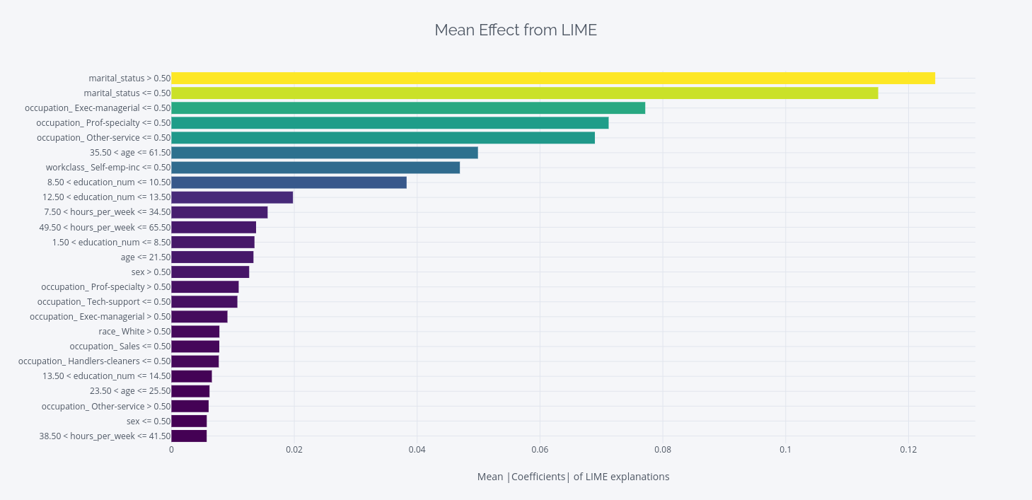
There are two charts where we have aggregated the explanations across the 500 points we sampled from out test set(we can run it on all test data points, but chose to do sampling only cause of computation).

The first chart aggregates the effect of the feature across >50k and <50k cases and ignores the sign when calculating the mean. This gives you an idea of what features were important in the larger sense.

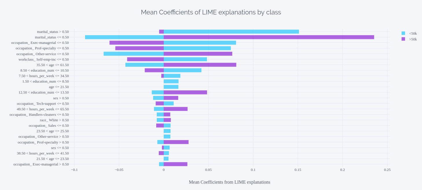
The second chart splits the inference across the two labels and looks at them separately. This chart lets us understand which feature was more important in predicting a particular class.

• Right at the top of the first chart, we can find “marital_status > 0.5“. According to our encoding, it means single. So being single is a very strong indicator towards whether you get more or less than 50k. But wait, being married is second in the list. How does that help us?
• If you look at the second chart, the picture is more clear. You can instantly see that being single, puts you in the <50k bucket and being married towards the >50k bucket.
• Before you rush off to find a partner, keep in mind that this is what the model is using to find it. It need not be the causation in the real world. Maybe the model is picking up on some other trait, which has a lot of correlation with getting married, to predict the earning potential.
• We can also observe the tinges of sexual discrimination here. If you look at “sex>0.5”, which is male, the distribution between the two earning potential classes is almost equal. But just take a look at the “sex<0.5”. It shows a large skew towards the <50k bucket.

Along with these, the submodular pick also (in fact, this is the main purpose of the module) a set of n data points from the dataset, which best explains the model. We can look at it as a representative sample of the different cases in the dataset. So if we need to explain a few cases from the model to someone, this gives you those cases which will cover the most ground.

THE JOKER IN THE PACK

From the looks of it, this looks like a very good technique, isn’t it? But it is not without its problems.

The biggest problem here is the correct definition of the neighbourhood, especially in tabular data. For images and text, it is more straightforward. Since the authors of the paper left kernel width as a hyperparameter, choosing the right one is left to the user. But how do you tune the parameter when you don’t have a ground truth? You’ll just have to try different widths, look at the explanations, and see if it makes sense. Tweak them again. But at what point are we crossing the line into tweaking the parameters to get the explanations we want?

Another main problem is similar to the problem we have with permutation importance (Part II). When sampling for the points in the locality, the current implementation of LIME uses a gaussian distribution, which ignores the relationship between the features. This can create the same ‘unlikely’ data points on which the explanation is learned.

And finally, the choice of a linear interpretable model for local explanations may not hold true for all the cases. If the decision boundary is too non-linear, the linear model might not explain it well(local fidelity may be high).

6) Shapely Values

Before we discuss how Shapely Values can be used for machine learning model explanation, let’s try to understand what they are. And for that, we have to take a brief detour into Game Theory.

Game Theory is one of the most fascinating branches of mathematics which deals with mathematical models of strategic interaction among rational decision-makers. When we say game, we do not mean just chess or, for that matter, monopoly. Game can be generalized into any situation where two or more players/parties are involved in a decision or series of decisions to better their position. When you look at it that way, it’s application extends to war strategies, economic strategies, poker games, pricing strategies, negotiations, and contracts. The list is endless.

But since our topic of focus is not Game Theory, we will just go over some major terms so that you’ll be able to follow the discussion. The parties participating in a Game are called Players. The different actions these players can take are called choices. If there is a finite set of choices for each player, there is also a finite set of combinations of choices of each player. So if each player plays a choice, it will result in an outcome, and if we quantify those outcomes, it’s called a payoff. And if we list all the combinations and the payoffs associated with it, it’s called payoff matrix.

There are two paradigms in Game Theory – Non-cooperative, Cooperative games. And Shapely values are an important concept in cooperative games. Let’s try to understand through an example.

Alice, Bob, and Celine share a meal. The bill came to be 90, but they didn’t want to go dutch. So to figure out what they each owe, they went to the same restaurant multiple times in different combinations and recorded how much the bill was.

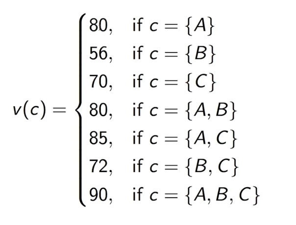
Now with this information, we do a small mental experiment. Suppose A goes to the restaurant, then B shows up and C shows up. So, for each person who joins, we can have the extra cash (marginal contribution) each person has to put in. We start with 80 (which is what A would have paid if he ate alone). Now when B joined, we look at the payoff when A and B ate together – also, 80. So the additional contribution B brought to the coalition is 0. And when C joined, the total payoff is 90. That makes the marginal contribution of C 10. So, the contribution when A, B, C joined in that order is (80,0,10). Now we repeat this experiment for all combinations of the three friends.

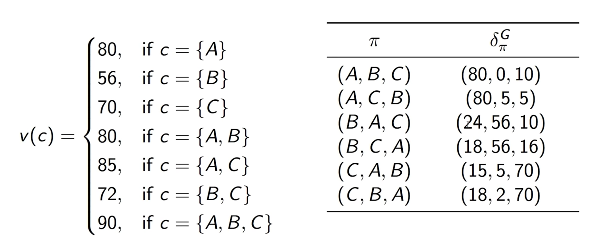
This is what you’ll get if you repeat the experiments for all orders of arriving.

Now that we have all possible orders of arriving, we have the marginal contributions of all the players in all situations. And the expected marginal contribution of each player is the average of their marginal contribution across all combinations. For example, the marginal contribution of A would be, (80+80+56+16+5+70)/6 = 51.17. And if we calculate the expected marginal contributions of each of the players and add them together, we will get 90- which is the total payoff if all three ate together.

You must be wondering what all these have to do with machine learning and interpretability. A lot. If we think about it, a machine learning prediction is like a game, where the different features (players), play together to bring an outcome (prediction). And since the features work together, with interactions between them, to make the prediction, this becomes a case of cooperative games. This is right up the alley of Shapely Values.

But there is just one problem. Calculating all possible coalitions and their outcomes quickly become infeasible as the features increase. Therefore, in 2013, Erik Štrumbelj et al. proposed an approximation using Monte-Carlo sampling. And in this construct, the payoff is modelled as the difference in predictions of different Monte-Carlo samples from the mean prediction.

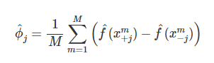
where f is the black box machine learning model we are trying to explain, x is the instance we are trying to explain, j is the feature for which we are trying to find the expected marginal contribution,  are two instances of x which we have permuted randomly by sampling another point from the dataset itself, and M is the number of samples we draw from the training set.

Let’s look at a few desirable mathematical properties of Shapely values, which makes it very desirable in interpretability application. Shapely Values is the only attribution method that satisfies the properties Efficiency, Symmetry, Dummy, and Additivity. And satisfying these together is considered to be the definition of a fair payout.

• Efficiency – The feature contributions add up to the difference in prediction for x and average.
• Symmetry – The contributions of two feature values should be the same if they contribute equally to all possible coalitions.
• Dummy – A feature that does not change the predicted value, regardless of which coalition it was added to, should have the Shapely value of 0
• Additivity – For a game with combined payouts, the respective Shapely values can be added together to get the final Shapely Value

While all of the properties make this a desirable way of feature attribution, one, in particular, has a far-reaching effect – Additivity. This means that for an ensemble model like a RandomForest or Gradient Boosting, this property guarantees that if we calculate the Shapely Values of the features for each tree individually and average them, you’ll get the Shapely values for the ensemble. This property can be extended to other ensemble techniques like model stacking or model averaging as well.

We will not be reviewing the algorithm and see the implementation of Shapely Values for two reasons:

• In most real-world applications, it is not feasible to calculate Shapely Values, even with the approximation.
• There exists a better way of calculating Shapely Values along with a stable library, which we will be covering next.

7) Shapely Additive Explanations (SHAP)

SHAP (SHapely Additive exPlanations) puts forward a unified approach to interpreting Model Predictions. Scott Lundberg et al. proposes a framework that unifies six previously existing feature attribution methods (including LIME and DeepLIFT) and they present their framework as an additive feature attribution model.

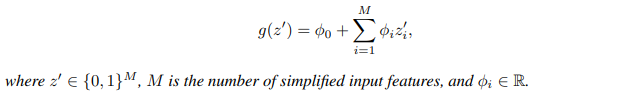
They show that each of these methods can be formulated as the equation above and the Shapely Values can be calculated easily, which brings with it a few guarantees. Even though the paper mentions slightly different properties than the Shapely Values, in principle, they are the same. This provides a strong theoretical foundation to the techniques(like LIME) once adapted to this framework of estimating the Shapely values. In the paper, the authors have proposed a novel model-agnostic way of approximating the Shapely Values called Kernel SHAP (LIME + Shapely Values) and some model-specific methods like DeepSHAP(which is the adaptation of DeepLIFT, a method for estimating feature importance for neural networks). In addition to it, they have also shown that for linear models, the Shapely Values can be approximated directly from the model’s weight coefficients, if we assume feature independence. And in 2018, Scott Lundberg et al. [6] proposed another extension to the framework which accurately calculates the Shapely values of tree-based ensembles like RandomForest or Gradient Boosting.

Kernel SHAP

Even though it’s not super intuitive from the equation below, LIME is also an additive feature attribution method. And for an additive feature explanation method, Scott Lundberg et al. showed that the only solution that satisfies the desired properties is the Shapely Values. And that solution depends on the Loss function L, weighting kernel  and regularization term .

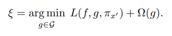
For easy reference. We have seen this equation before when we discussed LIME.

If you remember, when we discussed LIME, I mentioned that one of the disadvantages is that it left the kernel function and kernel distance as hyperparameters, and they are chosen using a heuristic. Kernel SHAP does away with that uncertainty by proposing a Shapely Kernel and a corresponding loss function which makes sure the solution to the equation above will result in Shapely values and enjoys the mathematical guarantees along with it.

ALGORITHM

• Sample a coalition vector (coalition vector is a vector of binary values of the same length as the number of features, which denotes whether a particular feature is included in the coalition or not.  (1 = feature present, 0 = feature absent)
• Get predictions from the model for the coalition vector  by converting the coalition vector to the original sample space using a function , which is just a fancy way of saying that we use one set of transformations to get the corresponding value from the original input data. For example, for all the 1’s in the coalition vector, we replace it by the actual value of that feature from the instance that we are explaining. And for the 0’s, it slightly differs according to the application. For Tabular data, 0’s are replaced with some other value of the same feature, randomly sampled from the data. For image data, 0’s can be replaced with a reference value or zero pixel value. The picture below tries to make this process clear for tabular data.
• Compute the weight of the sample using Shapely Kernel
• Repeat this for K samples
• Now, fit a weighted linear model and return the Shapely values, the coefficients of the model.

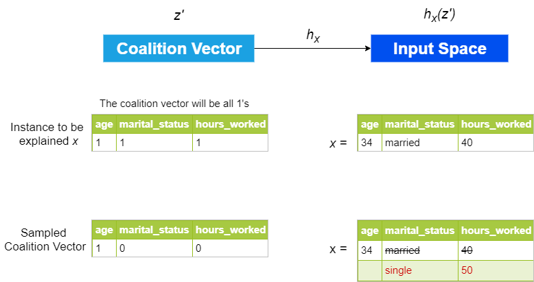
Representation of how the coalition vector is converted to original input space.

Tree SHAP

Tree SHAP, as mentioned before[6], is a fast algorithm that computes the exact Shapely Values for decision tree-based models. In comparison, Kernel SHAP only approximates the Shapely values and is much more expensive to compute.

ALGORITHM

Let’s try to get some intuition of how it is calculated, without going into a lot of mathematics(Those of you who are mathematically inclined, the paper is linked in the references, Have a blast!).

We will talk about how the algorithm works for a single tree first. If you remember the discussion about Shapely values, you will remember that to accurately calculate we need the predictions conditioned on all subsets of the feature vector of an instance. So let the feature vector of the instance we are trying to explain be x and the subset of feature for which we need the expected prediction to be S.

Below is an artificial Decision Tree that uses just three features, age, hours_worked, and marital_status to make the prediction about earning potential.

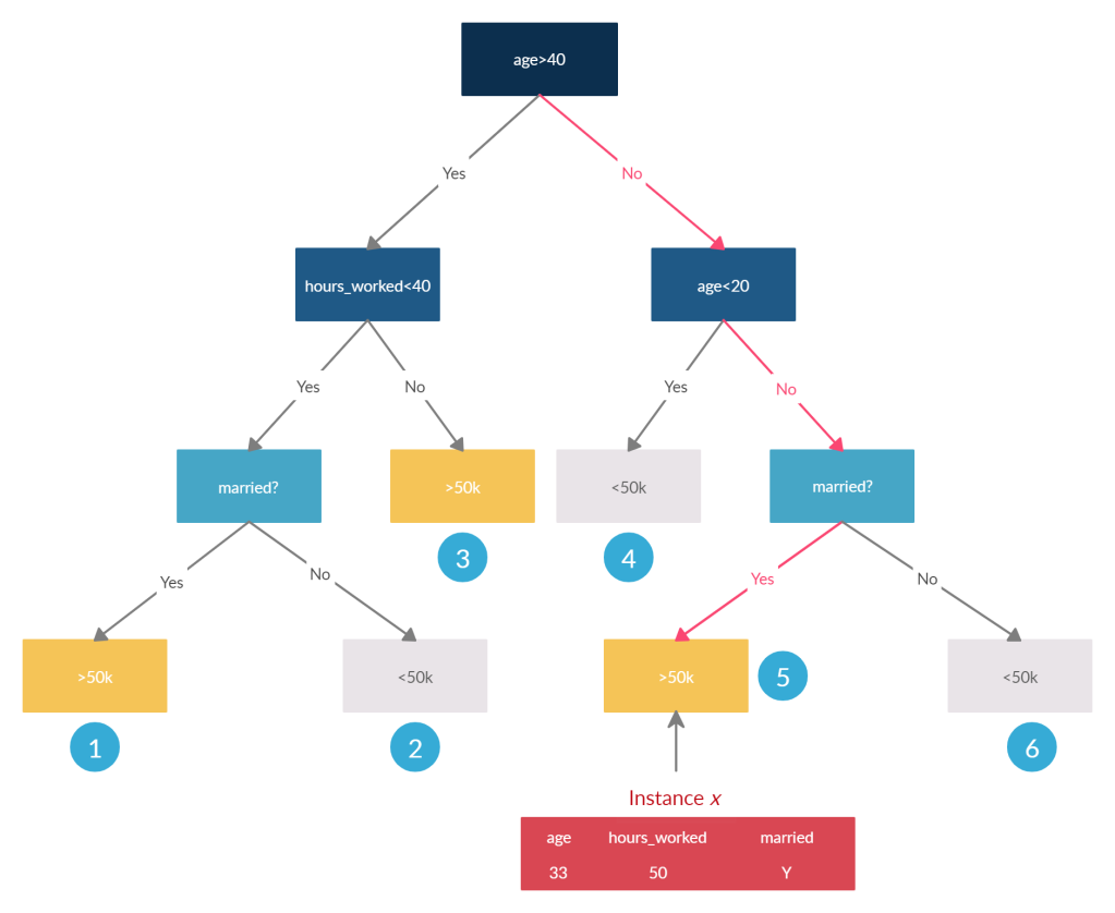
• If we condition on all features, i.e., Sis a set of all features, then the prediction in the node in which x falls in is the expected prediction. i.e. >50k
• If we condition on no features, it is equally likely(ignoring the distribution of points across nodes) that you end up in any of the decision nodes. And therefore, the expected prediction will be the weighted average of predictions of all terminal nodes. In our example, there are 3 nodes that output 1(<50k) and three nodes that output 0 (>50k). If we assume all the training data points were equally distributed across these nodes, the expected prediction in the absence of all features is 0.5
• If we condition on some features S, we calculate the expected value over nodes, which are equally likely for the instance x to end up in. For eg. if we exclude marital_statusfrom the set S, the instance is equally likely to end up in Node 5 or Node 6. So the expected prediction for such an S, would be the weighted average of the outputs of Node 5 and 6. So if we exclude hours_worked from S, would there be any change in expected predictions? No, because hours_worked is not in the decision path for the instance x.
• If we are excluding a feature that is at the root of the tree, like age, it will create multiple sub-trees. In this case, it will have two trees, one starting with the marriedblock on the right-hand side and another starting with hours_worked on the left-hand side. There will also be a decision stub with Node 4. And now the instance x is propagated down both the trees(excluding the decision path with age), and expected prediction is calculated as the weighted average of all the likely nodes(Nodes 3, 4 and 5).

And now that you have the expected predictions of all subsets in one Decision Tree, you repeat that for all the trees in an ensemble. And remember the additivity property of Shapely values? It lets you aggregate them across the trees in an ensemble by calculating an average of Shapely values across all the trees.

But, now the problem is that these expected values have to be calculated for all possible subsets of features in all the trees and all features. The authors of the paper proposed an algorithm, where we are able to push all possible subsets of features down the tree at the same time. The algorithm is quite complicated and I refer you to the paper linked in references to know the details.

ADVANTAGES

• SHAP and Shapely Values enjoy the solid theoretical foundation of Game Theory. And Shapely values guarantee that the prediction is fairly distributed across the different features. This might be the only feature attribution technique which will withstand the onslaught of theoretical and practical examination, be it academic or regulatory
• SHAP connects other interpretability techniques, like LIME and DeepLIFT, to the strong theoretical foundation of Game Theory.
• SHAP has a lightning-fast implementation for Tree-based models, which are one of the most popular sets of methods in Machine Learning.
• SHAP can also be used for global interpretation by calculating the Shapely values for a whole dataset and aggregating them. It provides a strong linkage between your local and global interpretation. If you use LIME or SHAP for local explanation and then rely on PDP plots to explain them globally, it does not really work out, and you might end up with conflicting inferences.

IMPLEMENTATION (LOCAL EXPLANATION)

We will only be looking at TreeSHAP in this section for two reasons:

1. We were looking at structural data all through the blog series and the model we chose to run the explainability techniques on is RandomForest, which is a tree-based ensemble.
2. TreeSHAP and KernelSHAP have pretty much the same interface in the implementation, and it should be pretty simple to swap out TreeSHAP with KernelSHAP (at the expense of computation) if you are trying to explain an SVM or some other model which is not tree-based.

import shap
 
# load JS visualization code to notebook
shap.initjs()
 
explainer = shap.TreeExplainer(model = rf, model_output='margin')
shap_values = explainer.shap_values(X_test)

These lines of code calculate the Shapely values. Even though the algorithm is fast, this will still take some time.

• In case of classification, the shap_valueswill be a list of arrays and the length of the list will be equal to the number of classes
• Same is the case with the expected_value
• So, we should choose which label we are trying to explain and use the corresponding shap_value and expected_value in further plots. Depending on the prediction of an instance, we can choose the corresponding SHAP values and plot them
• In case of a regression, the shap_values will only return a single item.

Now let’s look at individual explanations. We will take the same cases as LIME. There are multiple ways of plotting the individual explanations in SHAP library – Force Plots and Decision Plots. Both are very intuitive to understand the different features playing together to arrive at the prediction. If the number of features is too large, Decision Plots hold a slight advantage in interpreting.

shap.force_plot(
    base_value=explainer.expected_value[1],
    shap_values=shap_values[1][row],
    features=X_test.iloc[row],
    feature_names=X_test.columns,
    link="identity",
    out_names=">50k",
)
 
# We provide new_base_value as the cutoff probability for the classification mode
# This is done to increase the interpretability of the plot 
shap.decision_plot(
    base_value=explainer.expected_value[1],
    shap_values=shap_values[1][row],
    features=X_test.iloc[row],
    feature_names=X_test.columns.tolist(),
    link="identity",
    new_base_value=0.5,
)

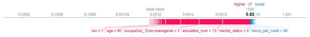
Force Plot.

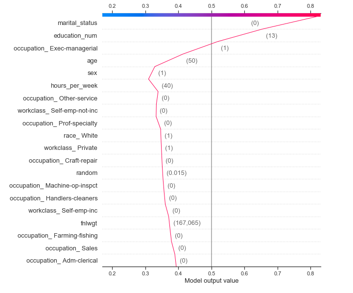
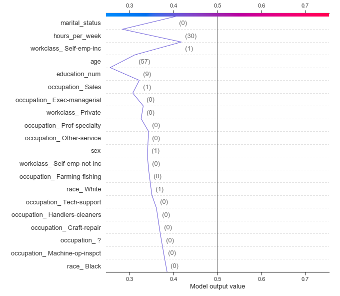
Decision Plot.

Now, we will check the second example.

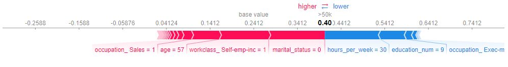
Force Plot.

INTERPRETATION

Example 1

• Similar to LIME, SHAP also attributes a large effect on marital_status, age, education_num, etc.
• The force plot explains how different features pushed and pulled on the output to move it from the base_valueto the prediction. The prediction here is the probability or likelihood that the person earns >50k (cause that is the prediction for the instance).
• In the force plot, you can see marital_status, education_num, etc. on the left-hand side pushing the prediction close to 1 and hours_per_week pushing in the other direction. We can see that from the base value of 0.24, the features have pushed and pulled to bring the output to 0.8
• In the decision plot, the picture is a little more clear. You have a lot of features like the occupation features and others which pushes the model output lower but strong influences from age, occupation_Exec-managerial, education_num, and marital_statushas moved the needle all the way till 0.8.
• These explanations fit our mental model of the process.

Example 2

• This is a case where we misclassified. And here the prediction we are explaining is that the person earned <50k, whereas they actually are earning >50k.
• The force plot shows an even match between both sides, but the model eventually converged to 0.6. The education, hours_worked, and the fact that this person is not in an exec-managerial role all tried to increase the likelihood of earning < 50k, because those were below average, whereas marital_status, the fact that he is self_employed, and his age, tried to decrease the likelihood.
• One more contributing factor, as you can see, are the base values(or priors). The model is starting with a prior that is biased towards <=50k because in the training data, that is the likelihood the model has observed. So the features have to work extra hard to make the model believe that the person earns >50k.
• This is more clear if you compare the decision plots of the two examples. In the second example, you can see a strong zig-zag pattern at the end where multiple strong influencers push and pull, resulting in less deviation from the prior belief.

IMPLEMENTATION (GLOBAL EXPLANATIONS)

The SHAP library also provides with easy ways to aggregate and plot the Shapely values for a set of points(in our case the test set) to have a global explanation for the model.

#Summary Plot as a bar chart
shap.summary_plot(shap_values = shap_values[1], features = X_test, max_display=20, plot_type='bar')
 
#Summary Plot as a dot chart
shap.summary_plot(shap_values = shap_values[1], features = X_test, max_display=20, plot_type='dot')
 
#Dependence Plots (analogous to PDP)
# create a SHAP dependence plot to show the effect of a single feature across the whole dataset
shap.dependence_plot("education_num", shap_values=shap_values[1], features=X_test)
 
shap.dependence_plot("age", shap_values=shap_values[1], features=X_test)

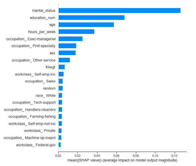
Summary Plot (Bar).

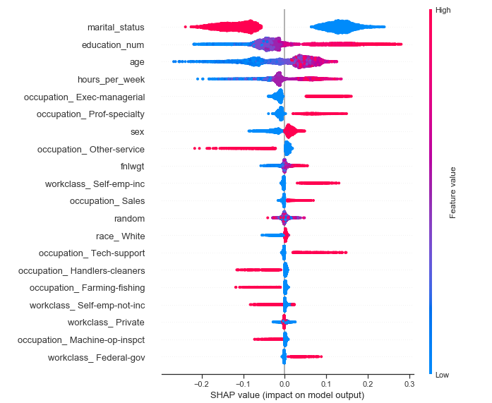
Summary Plot (Dot).

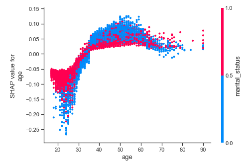
Dependence Plot – Age.

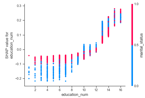
Dependence Plot – Education.

INTERPRETATION

• In binary classification, you can plot either of the two SHAP values that you get to interpret the model. We have chosen >50k to interpret because it is just more intuitive to think about the model that way
• In the aggregate summary, we can see the usual suspects at the top of the list.
  • Side note: we can provide a list of shap_values (multi-class classification) to the summary_plotmethod, provided we give plot_type = ‘bar.’ It will plot the summarized SHAP values for each class as a stacked bar chart. For binary classification, I found that to be much less intuitive than just plotting one of the classes.
• The Dot chart is much more interesting, as it reveals much more information than the bar chart. In addition to the overall importance, it also shows up how the feature value affects the impact on model output. For example, we can see clearly that marital_status gives a strong influence on the positive side(more likely to have >50k) when the feature value is low. And we know from our label encoding that marital_status = 0, means married and 1 means single. So being marriedincreases your chance of earning >50k.
  • Side note: We cannot use a list of shap values when using plot_type = ‘dot. You will have to plot multiple charts to understand each class you are predicting
• Similarly, if you look at age, you can see that when the feature value is low, almost always it contributes negatively to your chance of earning >50k. But when the feature value is high(i.e., you are older), there is a mixed bag of dots, which tells us that there is a lot of interaction effects with other features in making the decision for the model.
• This is where the dependence plotscome in to picture. The idea is very similar to PD plots we reviewed in the last blog post. But instead of partial dependence, we use the SHAP values to plot the dependence. The interpretation remains the similar with minor modifications.
• On the X-axis, it is the value of the feature, and on the Y-axis is the SHAP value or the impact it has on the model output. As you saw in the Dot chart, a positive impact means it is pushing the model output towards the prediction(>50k in our case) and negative means the other direction. So in the age dependence plot, we can see the same phenomenon we discussed earlier, but more clearly. When you are younger, the influence is mostly negative and when you are older the influence is positive.
• The dependence plot in SHAP also does one other thing. It picks another feature, which is having the most interaction with the feature we are investigating and colors the dots according to the feature value of that feature. In the case of age, it is marital_status that the method picked. And we can see that most of the dispersion you find on the age axis is explained by marital status.
• If we look at the dependence plot for education(which is an ordinal feature), we can see the expected trend of higher the education, better your chances of earning well.

JOKER IN THE PACK

As always, there are disadvantages that we should be aware of to effectively use the technique. If you were following along to find the perfect technique for explainability, I’m sorry to disappoint you. Nothing in life is perfect. So, let’s dive into the shortcomings.

• Computationally Intensive. TreeSHAP solves it to some extent, but it is still slow compared to most of the other techniques we discussed. KernelSHAP is just slow and becomes infeasible to calculate for larger datasets. (Although there are techniques like clustering using K-means to reduce the dataset before calculating the Shapely values, they are still slow)
• SHAP values can be misinterpretedas it is not the most intuitive of ideas. The concept that it represents not the actual difference in predictions, but the difference between actual prediction and mean predictions is a subtle nuance.
• SHAP does not create sparse explanationslike LIME. Humans prefer to have sparse explanations that fit well in the mental model. But adding a regularization term like what LIME does not guarantee Shapely values.
• KernelSHAP ignores feature dependence. Just like permutation importance, LIME, or any other permutation-based methods, KernelSHAP considers ‘unlikely’ samples when trying to explain the model.

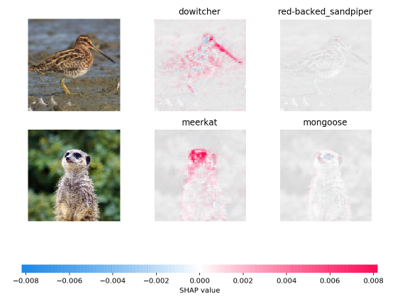
Bonus: Text and Image

Some of the techniques we discussed are also applicable to Text and Image data. Although we will not be going in deep, I’ll link to some notebooks which show you how to do it.

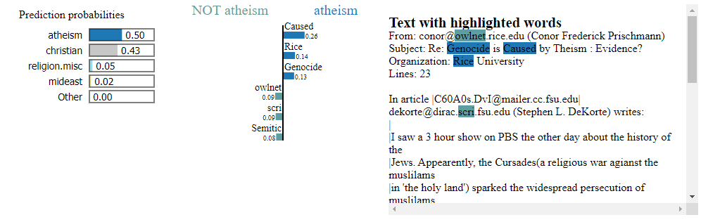
LIME ON TEXT DATA – MULTI-LABEL CLASSIFICATION

LIME ON IMAGE CLASSIFICATION – INCEPTION_V3 – KERAS

DEEP EXPLAINER – SHAP -MNIST

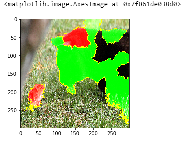
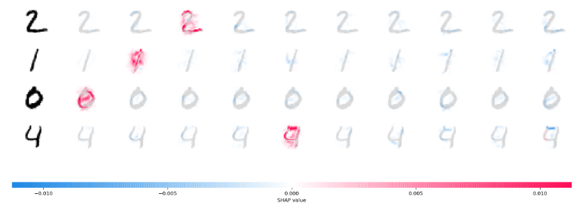
GRADIENT EXPLAINER – SHAP – INTERMEDIATE LAYER IN VGG16 IN IMAGENET

Final Words

We have come to the end of our journey through the world of explainability. Explainability and Interpretability are catalysts for business adoption of Machine Learning (including Deep Learning), and the onus is on us practitioners to make sure these aspects get addressed with reasonable effectiveness. It’ll be a long time before humans trust machines blindly and till then, we will have to supplant the excellent performance with some kind of explainability to develop trust.

If this series of blog posts enabled you to answer at least one question about your model, I consider my endeavor a success.

Full Code is available in my Github.

REFERENCES

1. Christoph Molnar, “Interpretable Machine Learning: A Guide for making black box models explainable"
2. Marco Tulio Ribeiro, Sameer Singh, Carlos Guestrin, “Why Should I Trust You?: Explaining the Predictions of Any Classifier”, arXiv:1602.04938 [cs.LG]
3. Shapley, Lloyd S. “A value for n-person games.” Contributions to the Theory of Games 2.28 (1953): 307-317
4. Štrumbelj, E., & Kononenko, I. (2013). Explaining prediction models and individual predictions with feature contributions. Knowledge and Information Systems, 41, 647-665.
5. Lundberg, Scott M., and Su-In Lee. "A unified approach to interpreting model predictions." Advances in Neural Information Processing Systems. 2017.
6. Lundberg, Scott M., Gabriel G. Erion, and Su-In Lee. “Consistent individualized feature attribution for tree ensembles.” arXiv preprint arXiv:1802.03888 (2018).

Original. Reposted with permission.

Bio: Manu Joseph (@manujosephv) is an inherently curious and self-taught Data Scientist with about 8+ years of professional experience working with Fortune 500 companies, including a researcher at Thoucentric Analytics.

Related:

• Explainability: Cracking open the black box, Part 1
• Interpretability: Cracking open the black box, Part 2
• “Please, explain.” Interpretability of machine learning models