Semi-supervised learning with Generative Adversarial Networks

By Tryambak Kaushik

This post is part of the "superblog" that is the collective work of the participants of the GAN workshop organized by Aggregate Intellect. This post serves as a proof of work, and covers some of the concepts covered in the workshop in addition to advanced concepts pursued by the participants.

Code:

• https://github.com/tryambak2019/SGAN

Papers Referenced:

• https://arxiv.org/abs/1606.01583

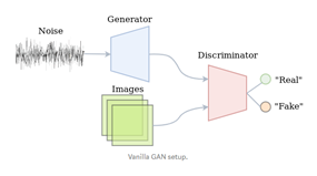
The original GAN (Goodfellow, 2014) (https://arxiv.org/abs/1406.2661) is a generative model, where a neural-network is trained to generate realistic images from random noisy input data. GANs generate predicted data by exploiting a competition between two neural networks, a generator (G) and a discriminator (D), where both networks are engaged in prediction tasks. G generates “fake” images from the input data, and D compares the predicted data (output from G) to the real data with results fed back to G. The cyclical loop between G and D is repeated several times to minimize the difference between predicted and ground truth data sets and improve the performance of G, i.e., D is used to improve the performance of G.

The paper discussed in this post, Semi-supervised learning with Generative Adversarial Networks (https://arxiv.org/abs/1606.01583), utilizes a GAN architecture for multi-label classification.

In order to demonstrate a proof of concept, the authors (Odena, 2016) use the MNIST image dataset. MNIST is a popular multi-label classification dataset and is extensively used to evaluate the performance of supervised learning algorithms in classifying dataset images into NN classes. Note that the authors used image datasets, but the concepts can be easily implemented for other datasets as well.

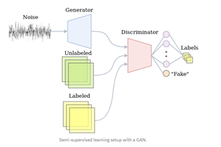
In the current GAN implementation, D classifies images into one of N + 1 classes, where NN is the number of pre-defined classes and 11 is the additional class to predict the class of output from G. In other words, D performs “supervised” classification of a given image with NN possible classes (or labels) and an “un-supervised” classification with 11 class to determine if the image is real or fake. G on the other hand generates increasingly realistic fake images which are fed to D, which forces D to improve its performance in determining if an image is real or fake, as well as classifying it into one of the MNIST labels. Thus, G is used to improve the performance of D in the current paper, which is a role that is reversed compared to original GAN paper. This implementation is defined as Semi-supervised Generative Adversarial Networks (SGAN).

Notes: Images from https://medium.com/@jos.vandewolfshaar/semi-supervised-learning-with-gans-23255865d0a4
 

The authors achieve this by replacing the sigmoid function in D with a softmax function.

The model is shown to improve classification performance, especially for small datasets, by up to 5 basis points above classification using simple convolution neural networks (CNNs) .

SGAN is also shown by the author to generate better predicted images than a regular GAN.

The discussion of SGAN henceforth is divided into the following sections:

1. Uploading and visualizing the data
2. Defining G and D
3. The training loop
4. Results

1. Uploading and visualizing the data

 
Pytorch libraries offer the MNIST data set and it can be easily loaded for the current analysis as follows:

train_set = dset.MNIST(root='./data', train=True, transform=trans)

The use of dset allows us to transform the raw dataset to resize, crop, change to the tensor data type, and normalize.

trans = transforms.Compose([transforms.Resize(image_size),

transforms.CenterCrop(image_size),

transforms.ToTensor(),

transforms.Normalize([0.5], [0.5])])

The MNIST training dataset has 6000 pairs of images and labels. Training the model on all these pairs simultaneously would require extensive computational resources. Therefore, the dataset is divided into many batches of a pre-defined small number of dataset pairs. This implementation requires less computational resources to train as the model trains only one batch at a time. Pytorch’s DataLoader offers a convenient way to create batches for training.

train_loader = torch.utils.data.DataLoader(

dataset=train_set,

batch_size=batch_size,

shuffle=True)

In order to verify its contents, the data-loader is iterated to display a batch of 25 images and labels.

2. Defining G and D

 
The Generator (G) of the adversarial network is used to upscale noisy data to a meaningful image. Upscaling in the current context refers to increasing the tensor dimensions of the noisy data (from n_zX1X1 to 1X28X28, where n_z is length of noise vector). In the current implementation, G consists of a linear layer followed by 3 hidden layers. Specifically, the hidden layers consist of 2 convolutional layers of type ConvTranspose2D with batch normalization, and 1 convolution layer without batch normalization. The logits output from the final convolution layer are activated with a tanh function.

The Discriminator (D) of the adversarial network, on the other hand, is used to downscale the image input to a pre-defined number of classes (or labels) of the classification problem. Opposite to upscaling, downscaling refers to decreasing the tensor dimensions (from 1X28X28 to 10X1X1). This downscaling is achieved with a combination of 3 hidden convolution layers of type Conv2D with batch normalization and 1 hidden linear layer.

The D of a semi-supervised GAN has two tasks: 1) Supervised learning and 2) Unsupervised learning. Hence, 2 activation functions, softmax and sigmoid, respectively, are defined within the GAN discriminator. The Softmax outputs 10 logits (for 10 possible output classes) for each image for multi-label classification, while the sigmoid outputs 1 logit to indicate a real or fake classification.

The loss function for supervised learning is also consequently defined as CrossEntropyLoss and BCELoss for supervised learning and semi-supervised learning, respectively.

Adam optimizer of stochastic gradient descent is used to update the weights of the neural network.

3. Training Loop

 
The training loop consists of two nested loops. The inner loop trains D and G over all the data batches defined earlier with DataLoader. The outer loop repeats this process on the training dataset 200 times (200 epochs).

The training within each loop is executed separately for supervised and unsupervised learning.

The unsupervised learning implementation is similar to a classical GAN, where the discriminator is trained on both real and fake data. Similar to a vanilla GAN, fake data is the output from the Generator (G) model, and it is fed as input into D model for binary (real/fake) classification.

However, the supervised learning implementation of SGAN is different from classical supervised learning algorithms, as SGAN models trains only on half MNIST training dataset, i.e., SGAN is able to achieve higher prediction accuracy by training only on half of the dataset. In fact, the nomenclature “Semi-supervised” learning derives itself from this modified GAN architecture. Furthermore, this implementation also prevents model overfitting as half of the training data set is not used to train the model.

The weights of G and D are initialized to a random normal distribution with zero mean and 0.02 standard deviation, before the start of training.

Binary Cross Entropy Loss function is used to calculate loss for G and unsupervised D, while Cross Entropy Loss function is used to calculate loss for supervised D. The total D loss, is thus, sum of supervised loss and unsupervised loss.

Adam optimizer is used to update the weights of D and G. The models are back propagated to implement the gradients and update the training weights at the end of each loop. However, to prevent gradient accumulation after each loop and avoid mix-up between mini-batches, the models are re-initialized as zero_grad() at the start of each loop.

After the model was trained on train dataset, it (the trained model D) was used to predict the image’s MNIST label for the test dataset.

4. Result Visualization

 
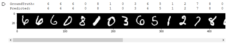
D performs extremely well in predicting labels of MNIST ‘test-dataset’, reaching an accuracy of 98%. The result is also very encouraging considering that only half of the training dataset was used to train D.

Further validating D‘s performance, predicted values match the groundtruth values of ‘train-dataset’ in the visual data comparison.

 
Original. Reposted with permission.

Related:

• Graduating in GANs: Going From Understanding Generative Adversarial Networks to Running Your Own
• Uber Creates Generative Teaching Networks to Better Train Deep Neural Networks
• Intro to Adversarial Machine Learning and Generative Adversarial Networks