 Deep Learning for Detecting Pneumonia from X-ray Images
 Deep Learning for Detecting Pneumonia from X-ray Images
This article covers an end to end pipeline for pneumonia detection from X-ray images.
The risk of pneumonia is immense for many, especially in developing nations where billions face energy poverty and rely on polluting forms of energy. The WHO estimates that over 4 million premature deaths occur annually from household air pollution-related diseases including pneumonia. Over 150 million people get infected with pneumonia on an annual basis especially children under 5 years old. In such regions, the problem can be further aggravated due to the dearth of medical resources and personnel. For example, in Africa’s 57 nations, a gap of 2.3 million doctors and nurses exists. For these populations, accurate and fast diagnosis means everything. It can guarantee timely access to treatment and save much needed time and money for those already experiencing poverty.
This project is a part of the Chest X-Ray Images (Pneumonia) held on Kaggle.
The Challenge
Build an algorithm to automatically identify whether a patient is suffering from pneumonia or not by looking at chest X-ray images. The algorithm had to be extremely accurate because lives of people is at stake.

Environment and tools
Data
The dataset can be downloaded from the kaggle website which can be found here.
Where is the code?
Without much ado, let’s get started with the code. The complete project on github can be found here.
Let’s start with loading all the libraries and dependencies.
Next I displayed some normal and pneumonia images to just have a look at how much different they look from the naked eye. Well not much!
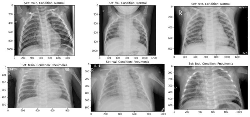
Then I split the data-set into three sets — train, validation and test sets.
Next I wrote a function in which I did some data augmentation, fed the training and test set images to the network. Also I created labels for the images.
The practice of data augmentation is an effective way to increase the size of the training set. Augmenting the training examples allow the network to “see” more diversified, but still representative, data points during training.
Then I defined a couple of data generators: one for training data, and the other for validation data. A data generator is capable of loading the required amount of data (a mini batch of images) directly from the source folder, convert them into training data (fed to the model) and training targets (a vector of attributes — the supervision signal).
For my experiments, I usually set the
batch_size = 64. In general a value between 32 and 128 should work well. Usually you should increase/decrease the batch size according to computational resources and model’s performances.
After that I defined some constants for later usage.
The next step was to build the model. This can be described in the following 5 steps.
- I used five convolutional blocks comprised of convolutional layer, max-pooling and batch-normalization.
- On top of it I used a flatten layer and followed it by four fully connected layers.
- Also in between I have used dropouts to reduce over-fitting.
- Activation function was Relu throughout except for the last layer where it was Sigmoid as this is a binary classification problem.
- I have used Adam as the optimizer and cross-entropy as the loss.
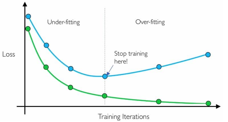
Before training the model is useful to define one or more callbacks. Pretty handy one, are: ModelCheckpoint and EarlyStopping.
- ModelCheckpoint: when training requires a lot of time to achieve a good result, often many iterations are required. In this case, it is better to save a copy of the best performing model only when an epoch that improves the metrics ends.
- EarlyStopping: sometimes, during training we can notice that the generalization gap (i.e. the difference between training and validation error) starts to increase, instead of decreasing. This is a symptom of overfitting that can be solved in many ways (reducing model capacity, increasing training data, data augumentation, regularization, dropout, etc). Often a practical and efficient solution is to stop training when the generalization gap is getting worse.
Next I trained the model for 10 epochs with a batch size of 32. Please note that usually a higher batch size gives better results but at the expense of higher computational burden. Some research also claim that there is an optimal batch size for best results which could be found by investing some time on hyper-parameter tuning.
Epoch 1/10
163/163 [==============================] - 90s 551ms/step - loss: 0.3855 - acc: 0.8196 - val_loss: 2.5884 - val_acc: 0.3783
Epoch 2/10
163/163 [==============================] - 82s 506ms/step - loss: 0.2928 - acc: 0.8735 - val_loss: 1.4988 - val_acc: 0.6284
Epoch 3/10
163/163 [==============================] - 81s 498ms/step - loss: 0.2581 - acc: 0.8963 - val_loss: 1.1351 - val_acc: 0.3970

Epoch 00003: ReduceLROnPlateau reducing learning rate to 0.0003000000142492354.
Epoch 4/10
163/163 [==============================] - 81s 495ms/step - loss: 0.2027 - acc: 0.9197 - val_loss: 0.3323 - val_acc: 0.8463
Epoch 5/10
163/163 [==============================] - 81s 500ms/step - loss: 0.1909 - acc: 0.9294 - val_loss: 0.2530 - val_acc: 0.9139

Epoch 00005: ReduceLROnPlateau reducing learning rate to 9.000000427477062e-05.
Epoch 6/10
163/163 [==============================] - 81s 495ms/step - loss: 0.1639 - acc: 0.9423 - val_loss: 0.3316 - val_acc: 0.8834
Epoch 7/10
163/163 [==============================] - 80s 492ms/step - loss: 0.1625 - acc: 0.9387 - val_loss: 0.2403 - val_acc: 0.8919

Epoch 00007: ReduceLROnPlateau reducing learning rate to 2.700000040931627e-05.
Epoch 8/10
163/163 [==============================] - 80s 490ms/step - loss: 0.1587 - acc: 0.9423 - val_loss: 0.2732 - val_acc: 0.9122
Epoch 9/10
163/163 [==============================] - 81s 496ms/step - loss: 0.1575 - acc: 0.9419 - val_loss: 0.2605 - val_acc: 0.9054

Epoch 00009: ReduceLROnPlateau reducing learning rate to 8.100000013655517e-06.
Epoch 10/10
163/163 [==============================] - 80s 490ms/step - loss: 0.1633 - acc: 0.9423 - val_loss: 0.2589 - val_acc: 0.9155
Let’s visualize the loss and accuracy plots.
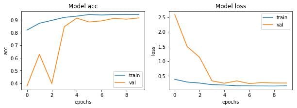
So far so good. The model is converging which can be observed from the decrease in loss and validation loss with epochs. Also it is able to reach 90% validation accuracy in just 10 epochs.
Let’s plot the confusion matrix and get some of the other results also like precision, recall, F1 score and accuracy.
CONFUSION MATRIX ------------------
[[191  43]
 [ 13 377]]

TEST METRICS ----------------------
Accuracy: 91.02564102564102%
Precision: 89.76190476190476%
Recall: 96.66666666666667%
F1-score: 93.08641975308642

TRAIN METRIC ----------------------
Train acc: 94.23
The model is able to achieve an accuracy of 91.02% which is quite good considering the size of data that is used.
Conclusions
Although this project is far from complete but it is remarkable to see the success of deep learning in such varied real world problems. I have demonstrated how to classify positive and negative pneumonia data from a collection of X-ray images. The model was made from scratch, which separates it from other methods that rely heavily on transfer learning approach. In the future this work could be extended to detect and classify X-ray images consisting of lung cancer and pneumonia. Distinguishing X-ray images that contain lung cancer and pneumonia has been a big issue in recent times, and our next approach should be to tackle this problem.
References/Further Readings
Training a CNN to detect Pneumonia
I remember the day so well. My grandfather started getting random coughs and began having trouble breathing. He was...
Detecting Pneumonia with Deep Learning
Pneumonia is lung inflammation caused by infection with virus, bacteria, fungi or other pathogens. According to...
CheXNet: Radiologist-Level Pneumonia Detection on Chest X-Rays with Deep Learning
The dataset, released by the NIH, contains 112,120 frontal-view X-ray images of 30,805 unique patients, annotated with...
Before You Go
The corresponding source code can be found here.
abhinavsagar/Kaggle-tutorial
Sample notebooks for Kaggle competitions. Automatic segmentation of microscopy images is an important task in medical...
Happy reading, happy learning and happy coding!
Contacts
If you want to keep updated with my latest articles and projects follow me on Medium. These are some of my contacts details:
Bio: Abhinav Sagar is a senior year undergrad at VIT Vellore. He is interested in data science, machine learning and their applications to real-world problems.
Original. Reposted with permission.
Related:
- Convolutional Neural Network for Breast Cancer Classification
- AI and Machine Learning for Healthcare
- How AI Can Help Manage Infectious Diseases