 Getting Started with TensorFlow 2
 Getting Started with TensorFlow 2
Learn about the latest version of TensorFlow with this hands-on walk-through of implementing a classification problem with deep learning, how to plot it, and how to improve its results.
But wait… What is Tensorflow?
Tensorflow is a Deep Learning Framework by Google, which released its 2nd version in 2019. It is one of the world's most famous Deep Learning frameworks widely used by Industry Specialists and Researchers.

Tensorflow v1 was difficult to use and understand as it was less Pythonic, but with v2 released with Keras now fully synchronized with Tensorflow.keras, it is easy to use, easy to learn, and simple to understand.
Remember, this is not a post on Deep Learning so I expect you to be aware of Deep Learning terms and the basic ideas behind it.
We will explore the world of Deep Learning with a very famous data set known as the IRIS data set.
Let’s jump straight into code to understand what is happening.
Importing and understanding the dataset
from sklearn.datasets import load_iris
iris = load_iris()
Now this iris is a dictionary. We can see it’s keys using
>>> iris.keys()
dict_keys([‘data’, ‘target’, ‘frame’, ‘target_names’, ‘DESCR’, ‘feature_names’, ‘filename’])
So our data is in data key, target is in target key, and so on. If you want to see details of this dataset, you can use iris['DESCR'].
Now we have to import other important libraries which will help us in creating our neural network.
from sklearn.model_selection import train_test_split #to split data

import numpy as np
import pandas as pd
import matplotlib.pyplot as plt

import tensorflow as tf
from tensorflow.keras.layers import Dense
from tensorflow.keras.models import Sequential
Here we have imported 2 main things from tensorflow, which are Dense and Sequential. Dense as we have imported it from tensorflow.keras.layers is a type of layer which is densely connected. The densely connected layer means that all nodes of previous layers are connected to all nodes of the current layers.
Sequential is an API from Keras commonly known as Sequential API that we will use to make our neural network.
To understand the data better, we can convert it into a data frame. Let’s do it.
X = pd.DataFrame(data = iris.data, columns = iris.feature_names)
print(X.head())
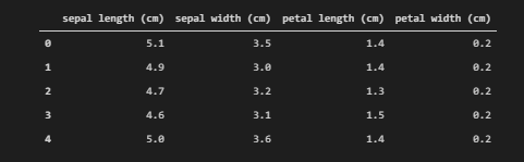
X.head()
Note that here we have set columns = iris.feature_names where feature_names is a key with the name of all 4 features.
Similarly for targets,
y = pd.DataFrame(data=iris.target, columns = [‘irisType’])
y.head()
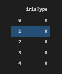
y.head()
To explore number of classes in our target set, we can use
y.irisType.value_counts()
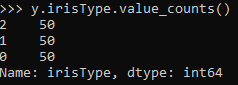
Here we can see that we have 3 classes, each with labels 0,1, and 2. To see the label name, we can use
iris.target_names #it is a key of dictionary iris
![]()
These are the names of the classes which we have to predict.
Data preprocessing for machine learning
Now, the first step for machine learning is data preprocessing. The main steps in data preprocessing are
- Filling missing values
- Splitting of data into training and validation sets
- Normalization of data
- Conversion of categorical data into one-hot vector
Missing values
To check if we have any missing values, we can use pandas.DataFrame.info() method to check.
X.info()
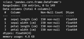
Here we can see that we have no missing value (luckily) and all our features are in float64.
Splitting into train and test sets
To split the data into the training and test sets, we can use train_test_split from sklearn.model_selection previously imported.
X_train, X_test, y_train, y_test = train_test_split(X,y, test_size=0.1)
where test_size is the argument that tells us that we want our test data to be 10% of the whole data.
Normalization of data
Typically, we normalize the data when we have a high amount of variance in it. To check the variance, we can use var() function from panadas.DataFrame to check var of all columns.
X_train.var(), X_test.var()
Here we can see that both X_train and X_test have very low variance, so no need to normalize the data.
Categorical data into one-hot vector
As we know that our output data is one of 3 classes already checked using iris.target_names, the good thing is that when we loaded the targets, they were already in 0, 1, 2 format where 0=1st class, 1=2nd class, and so on.
The problem with this representation is that our model might give higher numbers more priority, which can lead to results that are biased. So to tackle this, we are going to use one-hot representation. You can learn more about one-hot vectors here. We can either use the Keras built-in to_categorical or use OneHotEncoder from sklearn. We will use to_categorical.
y_train = tf.keras.utils.to_categorical(y_train)
y_test = tf.keras.utils.to_categorical(y_test)
We will review the first 5 rows only to check if it has converted it correctly or not.
y_train[:5,:]
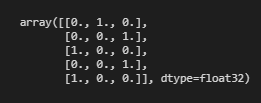
And yes, we have converted it into a one-hot representation.
One last thing
One last thing we can do is to convert our data back to numpy arrays so that we can use some extra functions that will help us later in our model. To do this we can use
X_train = X_train.values

X_test = X_test.values
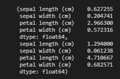
Let’s see what the result of the 1st training example.
X_train[0]
![]()
Here we can see the value of 4 features in the 1st training example, and its shape is (4,)
Our target labels were already in array format when we used to_categorical on them.
Machine learning model
Now finally, we are ready to create our model and train it. We will start from a simple model, and then we will go to complex model structures where we will cover different tips and techniques in Keras.
Lets code our basic model
model1 = Sequential() #Sequential Object
First, we have to create a Sequential Object. Now, to create a model, all we have to do is to add different types of layers as per our choice. We will make a 10 Dense layers model so that we can observe over-fitting, and reduce it later by different Regularization techniques.
model1.add( Dense( 64, activation = 'relu', input_shape= X_train[0].shape))
model1.add( Dense (128, activation = 'relu')
model1.add( Dense (128, activation = 'relu')
model1.add( Dense (128, activation = 'relu')
model1.add( Dense (128, activation = 'relu')
model1.add( Dense (64, activation = 'relu')
model1.add( Dense (64, activation = 'relu')
model1.add( Dense (64, activation = 'relu')
model1.add( Dense (64, activation = 'relu')
model1.add( Dense (3, activation = 'softmax')
Notice that in our first layer, we have used an extra argument of input_shape. This argument specifies the dimension of the first layer. We do not care about the number of training examples in this case. Instead, we only care about the number of features. So we pass in the shape of any training example, in our case, it was (4,) inside input_shape.
Notice that we have used softmax the activation function in our output layer because it is a multi-class classification problem. If it was a binary classification problem, we would have used sigmoid the activation function instead.
We can pass in any activation function we want such as sigmoid or linear or tanh, but it is proved via experiments that relu performs best in these kinds of models.
Now when we have defined the shape of our model, the next step is to specify it’s loss, optimizer, and metrics. We specify these using compile method in Keras.
model1.compile(optimizer='adam', loss= 'categorical_crossentropy', metrics = ['acc'])
Here we can use any optimizer such as Stochastic Gradient Descent, RMSProp, etc., but we will use Adam.
We are using categorical_crossentropy here because we have a multi-class classification problem, if we have a binary class classification problem, we would have used binary_crossentropy instead.
Metrics are important to evaluate one’s model. There are different metrics on the basis of which we can evaluate our model. For classification problems, the most important metric is accuracy, which tells how accurate our predictions are.
The last step in our model is to fit it on training data and training labels. Let's code it.
history = model1.fit(X_train, y_train, batch_size = 40, epochs=800, validation_split = 0.1
fit returns a callback that has all the history of our training, which we can use to do different useful tasks such as plotting etc.
History callback has an attribute named as history that we can access as history.history, which is a dictionary having all the history of losses and metrics, i.e., in our case, it has a history of loss, acc, val_loss, and val_acc and we can access every single one as history.history.loss or history.history['val_acc'] etc.
We have a specified number of epochs to 800, batch size to 40, and validation split to 0.1, meaning that we have now 10% validation data which we will use to analyze our training. Using 800 epochs will overfit the data, which means it will perform very well on training data, but not on testing data.
While the model is training, we can see our loss and accuracy both on the training and validation set.

Here we can see that our training accuracy is 100% and validation accuracy is 67% which is pretty good for such a model. Let’s plot it.
plt.plot(history.history['acc'])

plt.plot(history.history['val_acc'])

plt.xlabel('Epochs')

plt.ylabel('Acc')

plt.legend(['Training', 'Validation'], loc='upper right')
We can clearly see that accuracy for the training set is much higher than the accuracy for the validation set.
Similarly, we can plot Loss as
plt.plot(history.history['loss'])

plt.plot(history.history['val_loss'])

plt.xlabel('Epochs')

plt.ylabel('Loss')

plt.legend(['Training', 'Validation'], loc='upper left')
Here, we can clearly see that our Validation Loss is much higher than our Training Loss, which is because we have overfitted the data.
To check the model performance, we can use model.evaluate to check the performance of the model. We need to pass data and labels in evaluate method.
model1.evaluate(X_test, y_test)
Here, we can see that our model is giving 88% accuracy, which is pretty good for an overfitted model.
Regularization
Let’s make it better by adding regularization into our model. Regularization will reduce overfitting from our model and will improve our model.
We will add L2 regularization in our model. Learn more about L2 regularization here. To add L2 regularization in our model, we have to specify the layers, in which we want to add regularization and give an additional parameter which is kernel_regularizer, and pass tf.keras.regularizers.l2().
We will also implement some dropout in our model, which will help us reduce the overfitting better, and hence a better performing model. To read more about the theory and motivation behind dropout, refer to this article.
Let’s remake the model.
model2 = Sequential()
model2.add(Dense(64, activation = 'relu', input_shape= X_train[0].shape))
model2.add( Dense(128, activation = 'relu', kernel_regularizer=tf.keras.regularizers.l2(0.001)
))
model2.add( Dense (128, activation = 'relu',kernel_regularizer=tf.keras.regularizers.l2(0.001)
))
model2.add(tf.keras.layers.Dropout(0.5)
model2.add( Dense (128, activation = 'relu', kernel_regularizer=tf.keras.regularizers.l2(0.001)
))
model2.add(Dense(128, activation = 'relu', kernel_regularizer = tf.keras.regularizers.l2(0.001)

))
model2.add( Dense (64, activation = 'relu', kernel_regularizer=tf.keras.regularizers.l2(0.001)
))
model2.add( Dense (64, activation = 'relu', kernel_regularizer=tf.keras.regularizers.l2(0.001)
))
model2.add(tf.keras.layers.Dropout(0.5)
model2.add( Dense (64, activation = 'relu', kernel_regularizer=tf.keras.regularizers.l2(0.001)
))
model2.add( Dense (64, activation = 'relu', kernel_regularizer=tf.keras.regularizers.l2(0.001)
))
model2.add( Dense (3, activation = 'softmax', kernel_regularizer=tf.keras.regularizers.l2(0.001)
))
If you notice closely, we have all the layers and parameters the same except we have added 2 dropout layers and regularization in each dense layer.
We will keep all other things (loss, optimizer, epochs, etc.) the same.
model2.compile(optimizer='adam', loss='categorical_crossentropy', metrics=['acc'])
history2 = model2.fit(X_train, y_train, epochs=800, validation_split=0.1, batch_size=40)
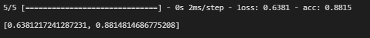
Let’s now evaluate the model.
model2.evaluate(X_test, y_test)

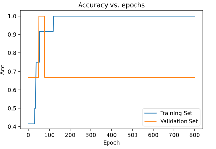
And guess what? We improved our accuracy from 88% to 94% just by adding regularization and dropout. If we add batch normalization to it, it will improve further.
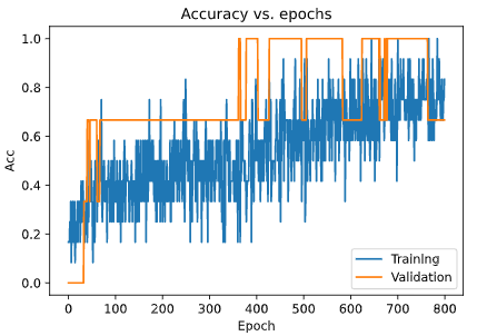
Let’s plot it.
Accuracy
plt.plot(history2.history['acc'])

plt.plot(history2.history['val_acc'])

plt.title('Accuracy vs. epochs')

plt.ylabel('Acc')

plt.xlabel('Epoch')

plt.legend(['Training', 'Validation'], loc='lower right')

plt.show()
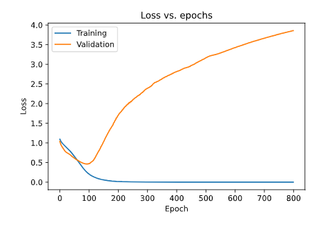
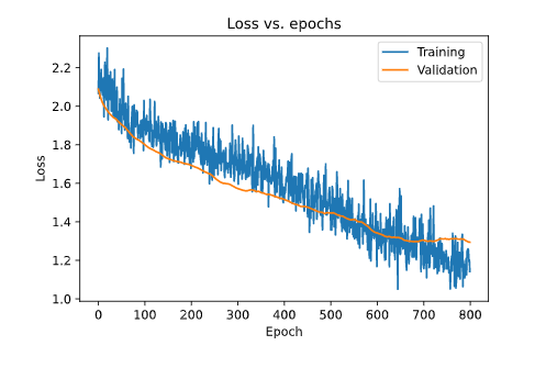
plt.plot(history2.history['loss'])

plt.plot(history2.history['val_loss'])

plt.title('Loss vs. epochs')

plt.ylabel('Loss')

plt.xlabel('Epoch')

plt.legend(['Training', 'Validation'], loc='upper right')

plt.show()
Insights
Here we can see that we have successfully removed the overfitting from over model, and improve our model by almost 6%, which is a good improvement for such a small dataset.
Related: