 Feature Engineering in SQL and Python: A Hybrid Approach
 Feature Engineering in SQL and Python: A Hybrid Approach
Set up your workstation, reduce workplace clutter, maintain a clean namespace, and effortlessly keep your dataset up-to-date.
By Shaw Lu, Data Scientist at Coupang

I knew SQL long before learning about Pandas, and I was intrigued by the way Pandas faithfully emulates SQL. Stereotypically, SQL is for analysts, who crunch data into informative reports, whereas Python is for data scientists, who use data to build (and overfit) models. Although they are almost functionally equivalent, I’d argue both tools are essential for a data scientist to work efficiently. From my experience with Pandas, I’ve noticed the following:
- I end up with many CSV files when exploring different features.
- When I aggregate over a big dataframe, the Jupyter kernel simply dies.
- I have multiple dataframes with confusing (and long) names in my kernel.
- My feature engineering codes look ugly and are scattered over many cells.
Those problems are naturally solved when I began feature engineering directly in SQL. So in this post, I’ll share some of my favorite tricks by working through a take-home challenge dataset. If you know a little bit of SQL, it’s time to put it into good use.
Installing MySQL
To start with, you need a SQL server. I’m using MySQL in this post. You can get MySQL server by installing one of the local desktop servers such as MAMP, WAMP or XAMPP. There are many tutorials online, and it’s worth going through the trouble.
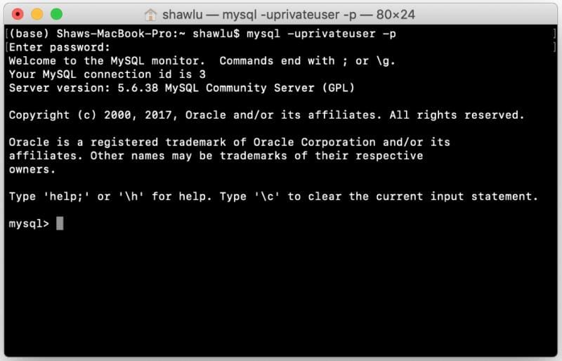
After setting up your server, make sure you have three items ready: username, password, port number. Login through Terminal by entering the following command (here we have username “root”, password 1234567).
mysql -uroot -p1234567
Then create a database called “Shutterfly” in the MySQL console (you can name it whatever you want). The two tables will be loaded into this database.
create database Shutterfly;
Install sqlalchemy
You’ll need Pandas and sqlalchemy to work with SQL in Python. I bet you already have Pandas. Then install sqlalchemy by activating your desired environment to launch Jupyter notebook, and enter:
pip install sqlalchemy
The sqlalchemy module also requires MySQLdb and mysqlclient modules. Depending on your OS, this can be installed using different commands.
Load Dataset into MySQL Server
In this example, we’ll load data from two CSV files, and engineer features directly in MySQL. To load datasets, we need to instantiate an engine object using username, password, port number, and database name. Two tables will be created: Online and Order. A natural index will be created on each table.
In MySQL console, you can verify that the tables have been created.
Split Dataset
This may seem counter-intuitive since we haven’t built any feature yet. But it’s actually very neat because all we need to do is to split dataset by index. By design, I also included the label (event 2) which we try to predict. When loading features, we will simply join the index with feature tables.
In MySQL console, you can verify that the training and test set are created.
Feature Engineering
This is the heavy lifting part. I write SQL code directly in Sublime Text, and debug my code by pasting them into MySQL console. Because this dataset is an event log, we must avoid leaking future information into each data point. As you can imagine, every feature needs to be aggregated over the history!
Joining table is the slowest operation, and so we want to get as many features as possible from each join. In this dataset, I implemented four types of join, resulting in four groups of features. The details are not important, but you can find all my SQL snippets here. Each snippet creates a table. The index is preserved and must match correctly to the response variable in the training set and test set. Each snippet is structured like this:
To generate the feature tables, open a new Terminal, navigate to the folder containing the sql files, and enter the following commands and passwords. The first snippet creates some necessary indices that speed up the join operation. The next four snippets create four feature tables. Without the indices, the joining takes forever. With the indices, it takes about 20 minutes (not bad on a local machine).
mysql < add_index.sql -uroot -p1234567
mysql < feature_group_1.sql -uroot -p1234567
mysql < feature_group_2.sql -uroot -p1234567
mysql < feature_group_3.sql -uroot -p1234567
mysql < feature_group_4.sql -uroot -p1234567
Now you should have the following tables in the database. Note that the derived features are stored separately from the original event logs, which help prevent confusion and disaster.
Load Features
Here I wrote a utility function that pulls data from the MySQL server.
- The function takes table name “trn_set” (training set) or “tst_set” (test set) as input, and an optional limit clause, if you only want a subset of the data.
- Unique columns, and columns with mostly missing values, are dropped.
- Date column is mapped to month, to help capture seasonality effect.
- Notice how the feature tables are joined in succession. This is actually efficient because we are always joining index on one-to-one mapping.
Finally, let’s take a look at 5 training examples, and their features.
Now you have a well-defined dataset and feature set. You can tweak the scale of each feature and missing values to suit your model’s requirement.
For tree-based methods, which are invariant to feature scaling, we can directly apply the model, and simply focus on tuning parameters! See an example of a plain-vanilla gradient boosting machine here.

It is nice to see that the useful features are all engineered, except for the category feature. Our efforts paid off! Also, the most predictive feature of event2 is how many nulls value were observed in event2. This is an illustrative case where we cannot replace null values by median or average, because the fact that they are missing is correlated with the response variable!
Summary
As you can see, we have no intermediate CSV files, a very clean namespace in our notebook, and our feature engineering codes are reduced to a few straightforward SQL statements. There are two situations in which the SQL approach is even more efficient:
- If your dataset is deployed on the cloud, you may be able to run distributed query. Most SQL server supports distirbuted query today. In Pandas, you need some extension called Dask DataFrame.
- If you can afford to pull data real-time, you can create SQL views instead of tables. In this way, every time you pull data in Python, your data will always be up-to-date.
One fundamental restriction of this approach is that you must be able to directly connect to your SQL server in Python. If this is not possible, you may have to download the query result as a CSV file and load it in Python.
I hope you find this post helpful. Though I’m not advocating method over another, it is necessary to understand the advantage and limitation of each method, and have both methods ready in our toolkit. So we can apply whichever method that works best under the constraints.
Bio: Shaw Lu is a Data Scientist at Coupang. He is an engineering graduate seeking to leverage data science to inform business management, supply chain optimization, growth marketing and operation research. Official author in Toward Data Science.
Original. Reposted with permission.
Related: