A Complete Guide To Survival Analysis In Python, part 3
Concluding this three-part series covering a step-by-step review of statistical survival analysis, we look at a detailed example implementing the Kaplan-Meier fitter based on different groups, a Log-Rank test, and Cox Regression, all with examples and shared code.
By Pratik Shukla, Aspiring machine learning engineer.
Index of the series
(1) Basics of survival analysis.
(2) Kaplan-Meier fitter theory with an example.
(3) Nelson-Aalen fitter theory with an example.
Part 3:
(4) Kaplan-Meier fitter based on different groups.
(5) Log-Rank Test with an example.
(6) Cox Regression with an example.
In the previous article, we saw how we could analyze the survival probability for patients. But it’s very important for us to know which factor affects survival most. So in this article, we discuss the Kaplan-Meier Estimator based on various groups.
Example 3: Kaplan-Meier Estimator with groups
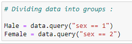
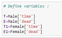
Let’s divide our data into 2 groups: Male and Female. Our goal here is to check is there any significant difference in survival rate if we divide our data set based on sex.
(1) Import required libraries:
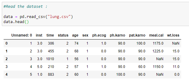
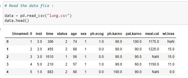
(2) Read the dataset:
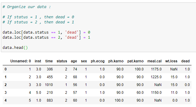
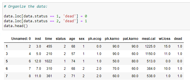
(3) Organize our data:
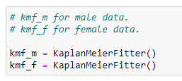
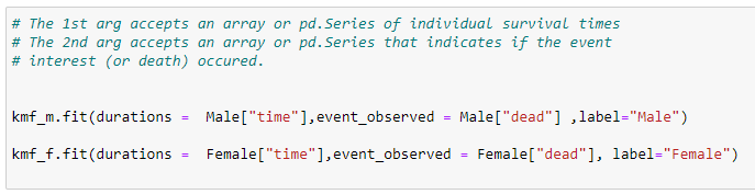
(4) Create two objects of KaplanMeierFitter():
kmf_m is for male dataset.
kmf_f is for female dataset.
(5) Divide data into groups:
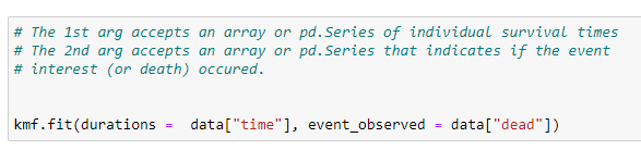
(6) Fit data into our objects:
(7) Generate event_tables:
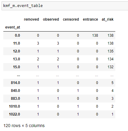
Event Table For Male.
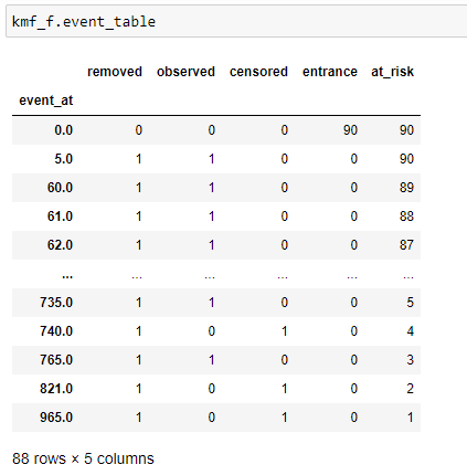
Event Table For Female.
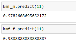
(7) Predicting survival probabilities:
Now we can predict the survival probability for both the groups.
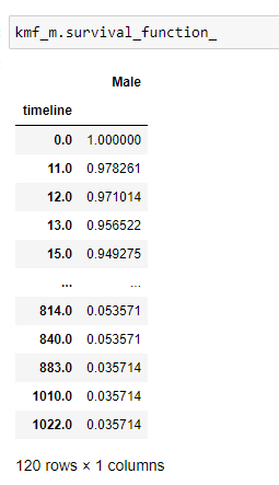
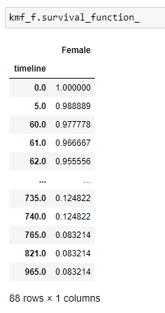
(8) Get the complete list of survival_probability:
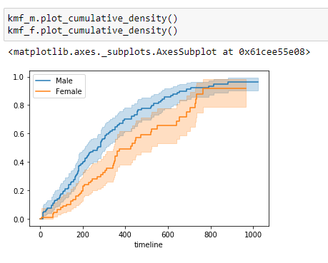
(9) Plot the graph:
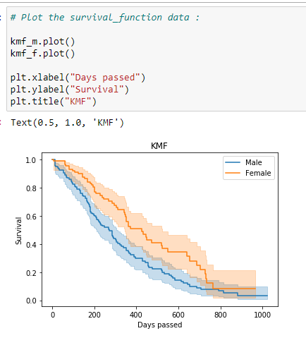
Notice that the probability of a female surviving lung cancer is higher than the probability of a male surviving lung cancer. So from this data, we can say that the medical researchers should focus more on the factors that lead to poor survival rates for male patients.
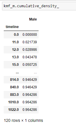
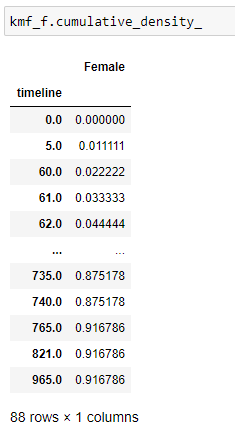
(10) Cumulitive_density:
It gives us a probability of a person dying at a certain timeline.
(11) Plot the data:
(12) Hazard function:
(13) Data fitting:
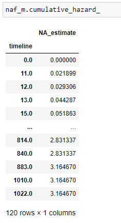
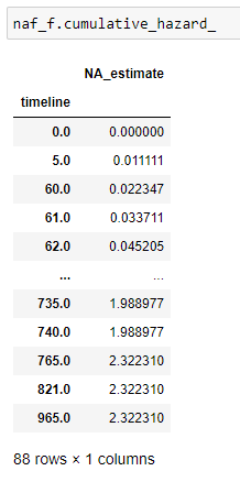
(14) Cumulative hazard:
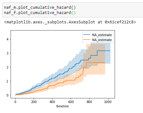
(15) Plot the data:
Log-Rank Test
Goal: Here, our goal is to see if there is any significant difference between the groups being compared.
Null Hypothesis: The null hypothesis states that there is no significant difference between the groups being studied. If there is a significant difference between these groups, then we have to reject our null hypothesis.
How do we say that there is a significant difference?
The statistical significance is denoted by a p-value between 0 and 1. The smaller the p-value, the greater the statistical difference between groups being studied. Notice that here our goal is to find if there is any difference between the groups we are comparing. If yes, then we can do more research on why there are lower survival chances for a particular group based on various information like their diet, lifestyle, etc.
Less than (5% = 0.05) P-value means that there is a significant difference between the groups that we compared. We can partition our groups based on their sex, age, race, method of treatment, etc.
It’s a test to find out the value of P.
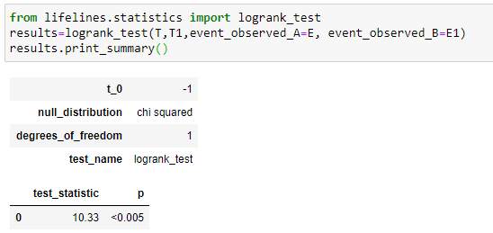
Here we’ll compare the survival distributions of two different groups by the famous statistical method of the log-rank test. Here notice that for our groups, the test_statistic equals 10.33, and the P-value indicates (<0.005), which is statistically significant and denotes that we have to reject our null hypothesis and admit that the survival function for both groups is significantly different. The P-value gives us strong evidence that “sex” was associated with survival days. In short, we can say that in our example, “sex” has a major contribution to survival days.
Putting it all together:
You can download the Jupyter notebooks from here.
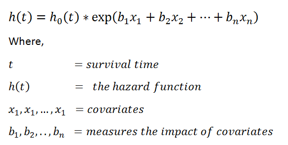
Example 4: Cox proportional hazard model
The Cox proportional hazard model is basically a regression model generally used by medical researchers to find out the relationship between the survival time of a subject and one or more predictor variables. In short, we want to find out how different parameters like age, sex, weight, height affects the length of survival for a subject.
In the previous section, we saw Kaplan-Meier, Nelson-Aalen, and Log-Rank Test. But in that, we were only able to consider one variable at a time. And one more thing to notice here is that we were performing operations only on categorical variables like sex, status, etc., which are not generally used for non-categorical data like age, weight, etc. As a solution, we use the Cox proportional hazards regression analysis, which works for both quantitative predictor (non-categorical) variables and categorical variables.
Why do we need it?
In medical research, generally, we are considering more than one factor to diagnose a person’s health or survival time, i.e., we generally make use of their sex, age, blood pressure, and blood sugar to find out if there is any significant difference between those in different groups. For example, if we are grouping our data based on a person’s age, then our goal will be to find out which age group has a higher survival chance. Is that the children’s group, adult’s group, or old person’s group? Now what we need to find is on what basis do we make the group? To find that we use Cox regression and find the coefficients of different parameters. Let’s see how that works!
Basics of the Cox proportional hazard method:
The ultimate purpose of the Cox proportional hazard method is to notice how different factors in our dataset impact the event of interest.
Hazard function:
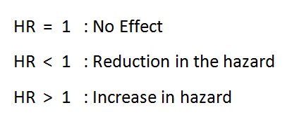
The values exp(bi) is called the hazard ratio (HR). The HR greater than 1 indicates that as the value of ith covariate increases, the event hazard increases, and thus the duration of survival decreases.
In summary,
Let’s code:
(1) Import required libraries:
(2) Read the CSV file:
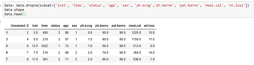
(3) Delete rows that contain null values:
Here we need to delete the rows which have null values. Our model can’t work on rows which has null values. If we don’t preprocess our data, then we might get an error.
(4) Create an object for KapanMeierFitter:

(5) Organize our data:
(6) Fit the values:
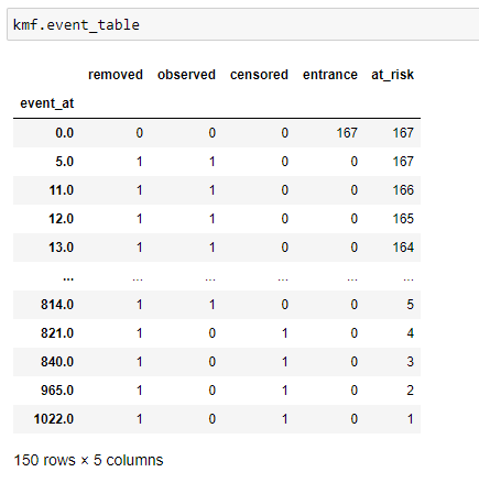
(7) Event table:
(8) Import Cox regression library:

(9) Parameters we want to consider while fitting our model:

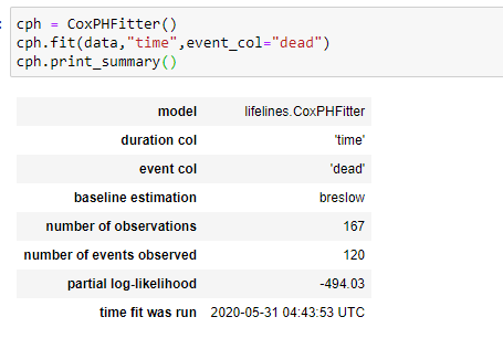
(10) Fit the data and print the summary:
Our model will consider all the parameters to find the coefficient values for that.
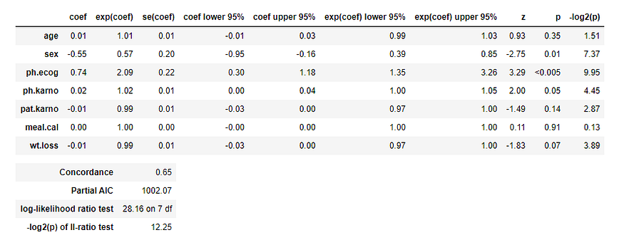
Here notice the p-value of different parameters as we know that a p-value (<0.05) is considered significant. Here you can see that the p-value of sex and ph.ecog are <0.05. So, we can say that we can group our data based on those parameters.
HR (Hazard Ratio) = exp(bi)
The p-value for sex is 0.01 and HR (Hazard Ratio) is 0.57 indicating a strong relationship between the patients’ sex and decreased risk of death. For example, holding the other covariates constant, being female (sex=2) reduces the hazard by a factor of 0.58, or 42%. That means that females have higher survival chances. Notice that we came to this conclusion using a graph in the previous section.
The p-value for ph.ecog is <0.005 and HR is 2.09, indicating a strong relationship between the ph.ecog value and increased risk of death. Holding the other covariates constant, a higher value of ph.ecog is associated with poor survival. Here person with higher ph.ecog value has a 109% higher risk of death. So, in short, we can say that doctors try to reduce the value of ph.ecog by providing relevant medicines.
Now notice that HR for Age is 1.01, which suggests only a 1% increase for the higher age group. So we can say that there is no significant difference between different age groups.
In short,
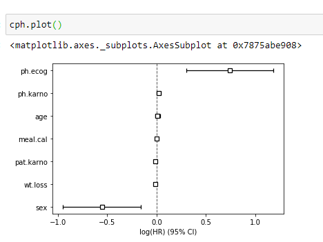
(11) Check which factor affects the most from the graph:
You can clearly see that ph.ecog and sex variables have significant differences.
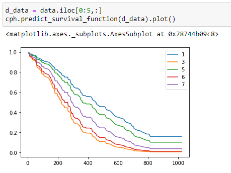
(12) Plot the graph:
Here I have plotted the survival probability for different persons in our dataset. Here notice that person-1 has the highest survival chances, and person-3 has the lowest survival chances. If you look at the main data, you can see that person-3 has a higher ph.ecog value.
Here notice that even if person-5 is alive, his/her survival probability is less since he/she has higher ph.ecog value.
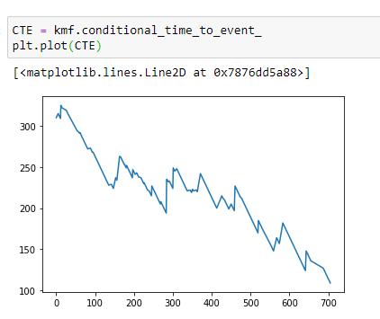
(13) Find out median time to event for timeline:
Here notice that as the number of days passed, the median survival time is decreasing.
Putting it all together:
You can download the Jupyter notebooks from here.
Original. Reposted with permission.
Bio: Pratik Shukla is an aspiring machine learning engineer who loves to put complex theories in simple ways. Pratik pursued his undergraduate in computer science and is going for a master's program in computer science at University of Southern California. “Shoot for the moon. Even if you miss it you will land among the stars. -- Les Brown”
Related: