Feature Ranking with Recursive Feature Elimination in Scikit-Learn
This article covers using scikit-learn to obtain the optimal number of features for your machine learning project.

Feature selection is an important task for any machine learning application. This is especially crucial when the data in question has many features. The optimal number of features also leads to improved model accuracy. Obtaining the most important features and the number of optimal features can be obtained via feature importance or feature ranking. In this piece, we’ll explore feature ranking.
Recursive Feature Elimination
The first item needed for recursive feature elimination is an estimator; for example, a linear model or a decision tree model.
These models have coefficients for linear models and feature importances in decision tree models. In selecting the optimal number of features, the estimator is trained and the features are selected via the coefficients, or via the feature importances. The least important features are removed. This process is repeated recursively until the optimal number of features is obtained.
Application in Sklearn
Scikit-learn makes it possible to implement recursive feature elimination via the sklearn.feature_selection.RFE class. The class takes the following parameters:
estimator— a machine learning estimator that can provide features importances via thecoef_orfeature_importances_attributes.n_features_to_select— the number of features to select. Selectshalfif it's not specified.step— an integer that indicates the number of features to be removed at each iteration, or a number between 0 and 1 to indicate the percentage of features to remove at each iteration.
Once fitted, the following attributes can be obtained:
ranking_— the ranking of the features.n_features_— the number of features that have been selected.support_— an array that indicates whether or not a feature was selected.
Application
As noted earlier, we’ll need to work with an estimator that offers a feature_importance_s attribute or a coeff_ attribute. Let’s work through a quick example. The dataset has 13 features—we’ll work on getting the optimal number of features.
import pandas as pddf = pd.read_csv(‘heart.csv’)df.head()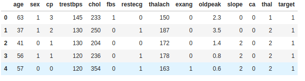
Let’s obtain the X and y features.
X = df.drop([‘target’],axis=1)
y = df[‘target’]
We’ll split it into a testing and training set to prepare for modeling:
from sklearn.model_selection import train_test_split
X_train, X_test, y_train, y_test = train_test_split(X, y,random_state=0)
Let’s get a couple of imports out of the way:
Pipeline— since we’ll perform some cross-validation. It’s best practice in order to avoid data leakage.RepeatedStratifiedKFold— for repeated stratified cross-validation.cross_val_score— for evaluating the score on cross-validation.GradientBoostingClassifier— the estimator we’ll use.numpy— so that we can compute the mean of the scores.
from sklearn.pipeline import Pipeline
from sklearn.model_selection import RepeatedStratifiedKFold
from sklearn.model_selection import cross_val_score
from sklearn.feature_selection import RFE
import numpy as np
from sklearn.ensemble import GradientBoostingClassifier
The first step is to create an instance of the RFE class while specifying the estimator and the number of features you’d like to select. In this case, we’re selecting 6:
rfe = RFE(estimator=GradientBoostingClassifier(), n_features_to_select=6)Next, we create an instance of the model we’d like to use:
model = GradientBoostingClassifier()We’ll use a Pipeline to transform the data. In the Pipeline we specify rfe for the feature selection step and the model that’ll be used in the next step.
We then specify a RepeatedStratifiedKFold with 10 splits and 5 repeats. The stratified K fold ensures that the number of samples from each class is well balanced in each fold. RepeatedStratifiedKFold repeats the stratified K fold the specified number of times, with a different randomization in each repetition.
pipe = Pipeline([(‘Feature Selection’, rfe), (‘Model’, model)])
cv = RepeatedStratifiedKFold(n_splits=10, n_repeats=5, random_state=36851234)
n_scores = cross_val_score(pipe, X_train, y_train, scoring=’accuracy’, cv=cv, n_jobs=-1)
np.mean(n_scores)
The next step is to fit this pipeline to the dataset.
pipe.fit(X_train, y_train)With that in place, we can check the support and the ranking. The support indicates whether or not a feature was chosen.
rfe.support_
array([ True, False,  True, False,  True, False, False,  True, False,True, False,  True,  True])
We can put that into a dataframe and check the result.
pd.DataFrame(rfe.support_,index=X.columns,columns=[‘Rank’])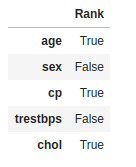
We can also check the relative rankings.
rf_df = pd.DataFrame(rfe.ranking_,index=X.columns,columns=[‘Rank’]).sort_values(by=’Rank’,ascending=True)rf_df.head()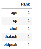
Automatic Feature Selection
Instead of manually configuring the number of features, it would be very nice if we could automatically select them. This can be achieved via recursive feature elimination and cross-validation. This is done via the sklearn.feature_selection.RFECV class. The class takes the following parameters:
estimator— similar to theRFEclass.min_features_to_select— the minimum number of features to be selected.cv— the cross-validation splitting strategy.
The attributes returned are:
n_features_— the optimal number of features selected via cross-validation.support_— the array containing information on the selection of a feature.ranking_— the ranking of the features.grid_scores_— the scores obtained from cross-validation.
The first step is to import the class and create its instance.
from sklearn.feature_selection import RFECVrfecv = RFECV(estimator=GradientBoostingClassifier())The next step is to specify the pipeline and the cv. In this pipeline we use the just created rfecv.
pipeline = Pipeline([(‘Feature Selection’, rfecv), (‘Model’, model)])
cv = RepeatedStratifiedKFold(n_splits=10, n_repeats=5, random_state=36851234)
n_scores = cross_val_score(pipeline, X_train, y_train, scoring=’accuracy’, cv=cv, n_jobs=-1)
np.mean(n_scores)
Let’s fit the pipeline and then obtain the optimal number of features.
pipeline.fit(X_train,y_train)The optimal number of features can be obtained via the n_features_ attribute.
print(“Optimal number of features : %d” % rfecv.n_features_)Optimal number of features : 7The rankings and support can be obtained just like last time.
rfecv.support_rfecv_df = pd.DataFrame(rfecv.ranking_,index=X.columns,columns=[‘Rank’]).sort_values(by=’Rank’,ascending=True)
rfecv_df.head()
With the grid_scores_ we can plot a graph showing the cross-validated scores.
import matplotlib.pyplot as plt
plt.figure(figsize=(12,6))
plt.xlabel(“Number of features selected”)
plt.ylabel(“Cross validation score (nb of correct classifications)”)
plt.plot(range(1, len(rfecv.grid_scores_) + 1), rfecv.grid_scores_)
plt.show()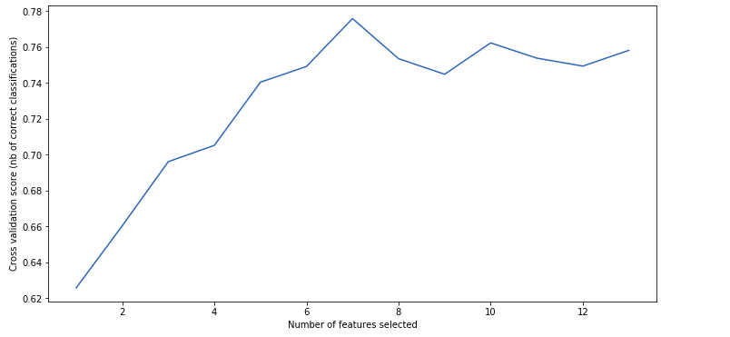
Final Thoughts
The process for applying this in a regression problem is the same. Just ensure to use regression metrics instead of accuracy. I hope this piece has given you some insight on selecting the optimal number of features for your machine learning problems.
mwitiderrick/Feature-Ranking-with-Recursive-Feature-Elimination
Feature Ranking with Recursive Feature Elimination - mwitiderrick/Feature-Ranking-with-Recursive-Feature-Elimination
Bio: Derrick Mwiti is a data analyst, a writer, and a mentor. He is driven by delivering great results in every task, and is a mentor at Lapid Leaders Africa.
Original. Reposted with permission.
Related:
- How I Consistently Improve My Machine Learning Models From 80% to Over 90% Accuracy
- LightGBM: A Highly-Efficient Gradient Boosting Decision Tree
- Fast Gradient Boosting with CatBoost